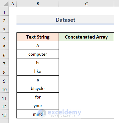
Method 1 – Concatenate a Single Array in Excel
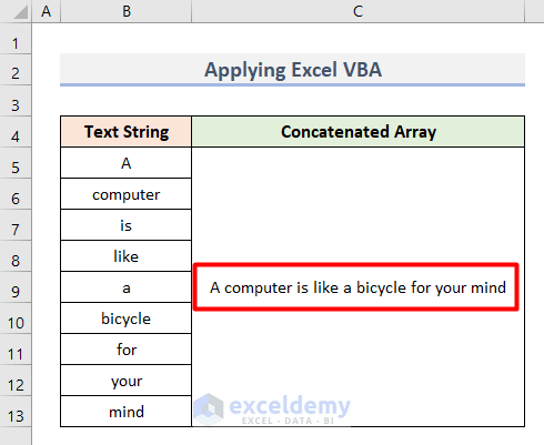
We will concatenate a single array from rows of a text string. We have a text string in the cell range B5:B13.
Case 1.1 – Combine CONCATENATE and TRANSPOSE Functions
- Select cell C8 and insert this formula.
=TRANSPOSE(B5:B13)&” “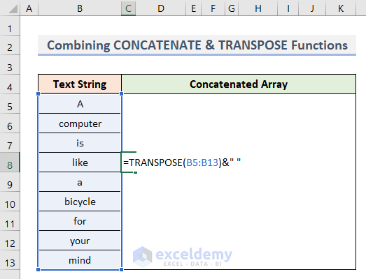
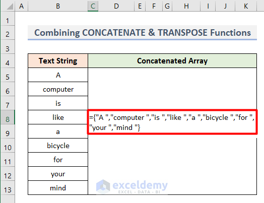
- Select the whole formula and press F9 on your keyboard to convert the formula into values.
- Add the CONCATENATE function at the beginning and complete the formula as follows.
=CONCATENATE("A ","computer ","is ","like ","a ","bicycle ","for ","your ","mind ")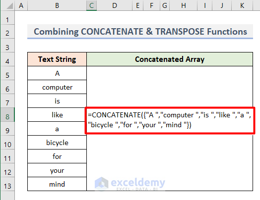
Note: On older versions, press Ctrl + Shift + Enter to use an array formula.
- Press Enter and you will see the required output.
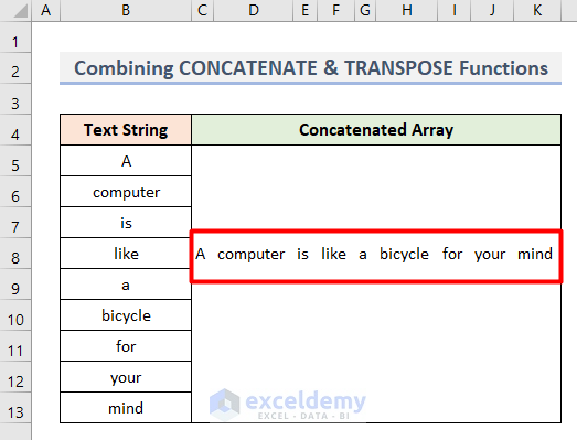
In this formula, the TRANSPOSE function converts the vertical cell range B5:B13 into a horizontal one. Following, the CONCATENATE function combines them and converts them to a single line.
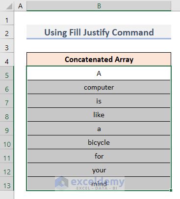
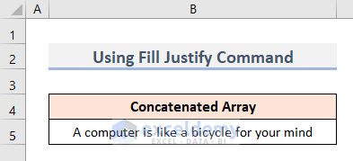
Case 1.2 -Use the Fill Justify Command in Excel
- Select cell range B5:B13.
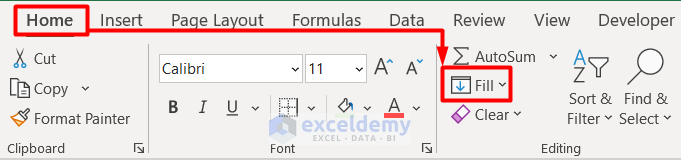
- Go to the Home tab and click on Fill under the Editing group.
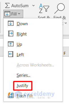
- Select Justify from the drop-down menu.
- You will get the concatenated array.
Case 1.3 – Apply the TEXTJOIN Function
- Select cell C9.
- Insert this formula.
=TEXTJOIN(" ",TRUE,B5:B13)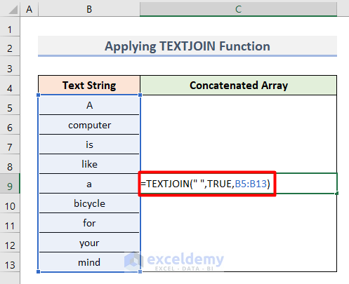
- Press Enter.
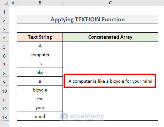
The TEXTJOIN function combines the text string into a single line. To get them with separators, we provided a space between two Quotation Marks (“)in the formula. Lastly, type TRUE along with the cell range B5:B13 to ignore empty cells from the dataset.
Case 1.4 – Concatenate with Power Query
- Select the cell range B5:B13.
- Go to the Data tab and select From Table/Range under Get & Transform Data.

- You will get the Power Query Editor window.
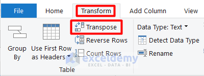
- Select the column and go to the Transform tab.
- Select Transpose from the Table group.
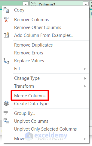
- Select all the separated columns in the window and right-click on any of them.
- Click on Merge Columns.
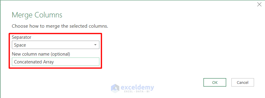
- Choose Space as the Separator in the Merge Columns dialogue box.
- Type Concatenated Array in the New column name section.
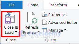
- Select Close & Load from the Home tab.
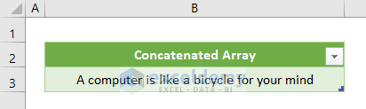
- You get the array in a new worksheet.
Case 1.5 – Apply Excel VBA Code
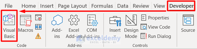
- Go to the Developer tab and select Visual Basic from the Code group.
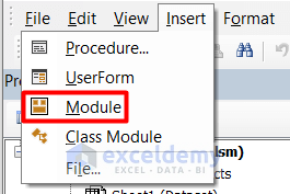
- Select Module from the Insert section in the Visual Basic window.
- Insert this code in the blank page.
Sub ConcatenateArray()
 Dim rg As Range
 Dim x As String
 For Each rg In Selection
 x = x & rg & " "
 Next rg
 Range("C9").Value = Trim(x)
 End Sub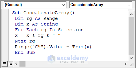
Note: The cell reference C9 is the location where you want to get the output. This cell reference can vary.
- Save the code and close the window.
- Select the cell range B5:B13.
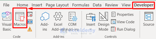
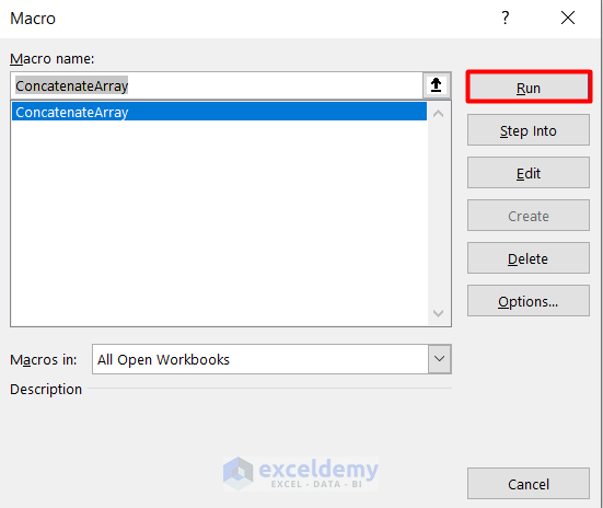
- Go to the Developer tab and click on Macros.
- You will get the Macros window with the Macro name.
- Click on Run.
- You’ll get the concatenated array.
Method 2 – Concatenate Multiple Arrays with Excel Formulas
Case 2.1 – Apply CHOOSE Function
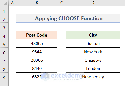
- Create a sample dataset with 5 City names and their Post Codes like the image below.
- Create a new table where we will get the output.
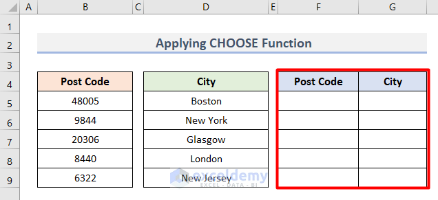
- Insert this formula in cell F5.
=CHOOSE({1,2},B5:B9,D5:D9)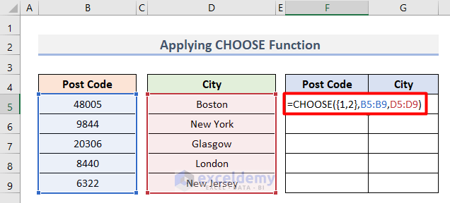
- Hit Enter and you will get the multiple arrays all at once.
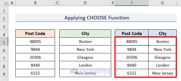
The CHOOSE function returns the values from the cell range B5:B9 and D5:D9.
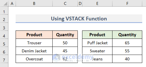
Case 2.2 – Use the Excel VSTACK Function for Vertical Concatenation
Here is a dataset with 6 Product names and Quantities in two different tables.
- Create a new table where you wish to get the output.
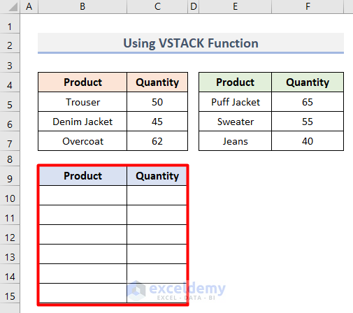
- Insert this formula in cell B10.
=VSTACK(B5:C7,E5:F7)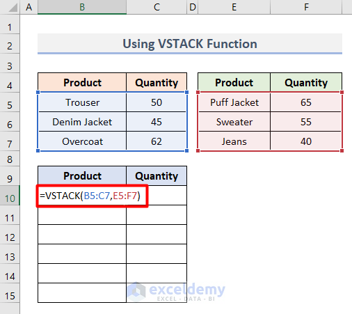
- Hit Enter. The arrays will “vertically stack” on top of each other.
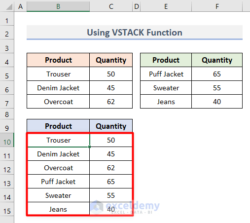
The VSTACK function helps to combine two individual datasets in the cell range B5:C7 and E5:F7 and transfer them into a vertical array.
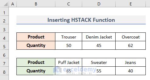
Case 2.3 – Insert HSTACK Function
- We will use the same dataset as before but arrange values horizontally.
- Insert this formula in cell C10.
=HSTACK(C4:E5,C7:E8)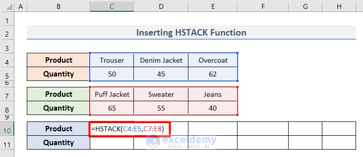
- Hit Enter. The arrays become stacked.
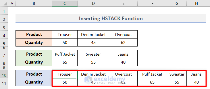
The HSTACK function helps to combine two individual datasets in the cell range C4:E5 and C7:E8 and transfer them into a horizontal array.
Things to Remember
- You can use the CONCAT function instead of the CONCATENATE function as well.
- The function accepts up to 255 text strings.
- Make sure there is no invalid argument in any of the formulas we described above. Otherwise, it will give you #Value! Error.
- In the case of the dynamic array, you must insert any of the formulas above in the leftmost cell of your output table. It will then automatically spill the array according to the formula.
Download the Practice Workbook
<< Go Back to Range | Concatenate | Learn Excel
Get FREE Advanced Excel Exercises with Solutions!
