How to Clear Pivot Cache in Excel (3 Effective Ways)

Method 1 – Using PivotTable Options

In this method, we will apply the PivotTable Options to clear the Pivot Cache. We will delete some of the data from the source data table after we insert the PivotTable. Then, we will clear the cache using the PivotTable Options.

Steps:

• Select the B5:D12 cell range.
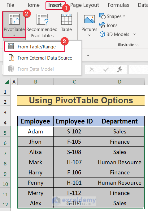
• Go to Insert.
• Choose PivotTable.
• From the drop-down options, choose From Table/Range.

• In the prompt, choose the B4:D12 cell range as the Table/Range.
• Check Existing Worksheet.
• Choose the F4 cell as the Location for the PivotTable.
• Click OK.

• Drag the Department, Employee and Employee ID fields under the Columns, Rows and Values options respectively.

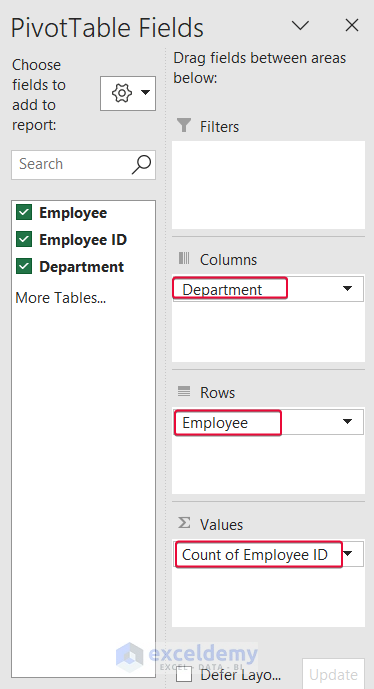
• The PivotTable will be inserted.

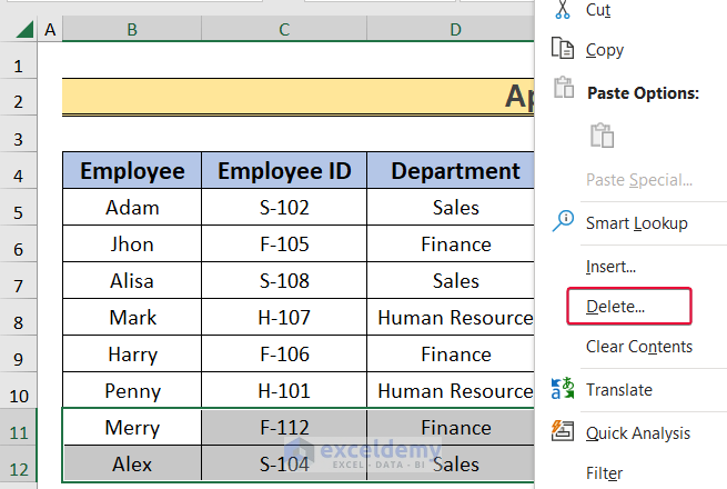
• Select the B11:D12 cell range and right-click.
• From the available options, choose Delete.

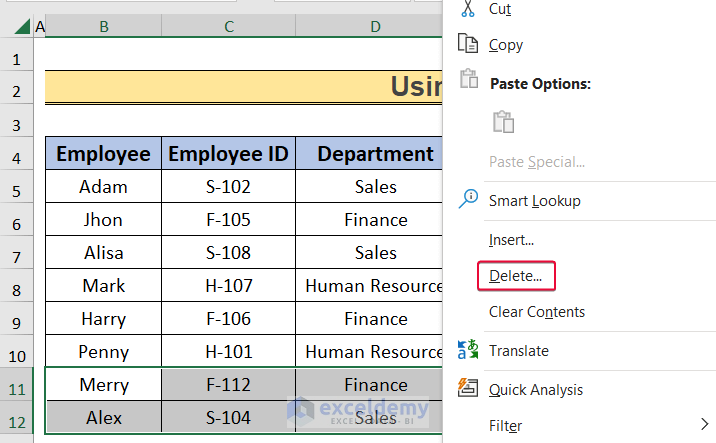
• In the pop-up dialog box, choose the Shift cells up option and click OK.

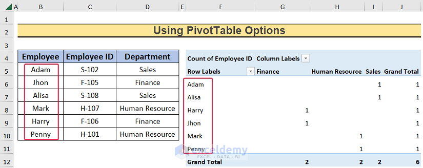
• The cells will be deleted from the data source.
• However, they are still in the PivotTable because of the PivotTable Cache.

• Select any of the cells on the PivotTable and right-click.
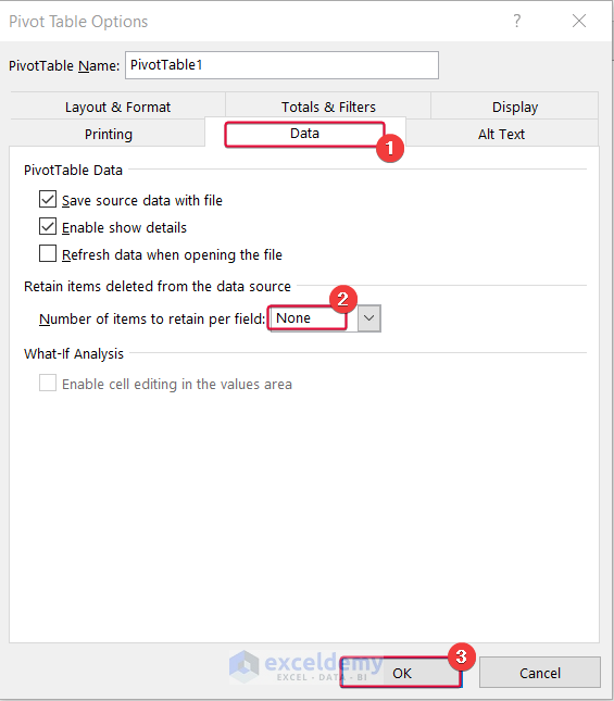
• From the available options, choose PivotTable Options.

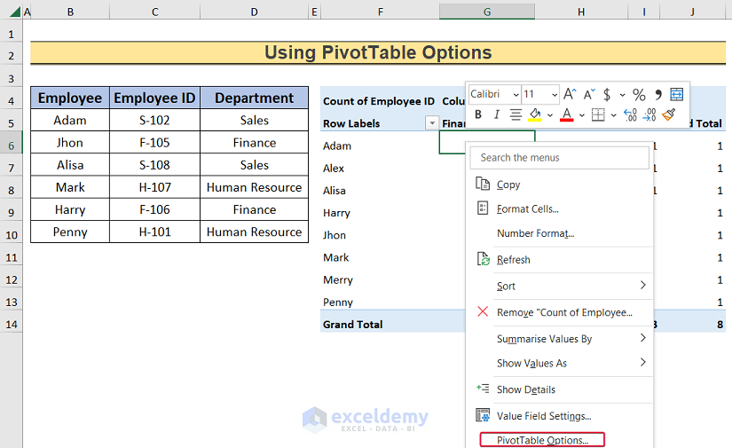
• In the prompt, go to the Data tab.
• From the Number of items to retain per field option, choose None.
• Click OK.

• Right-click on one of the data in the PivotTable.
• From the options, select Refresh.

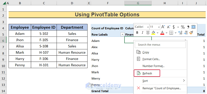
• The PivotTable will be updated according to the data source.

The Pivot Cache has been cleared.

Method 2 – Applying Excel VBA to Clear Pivot Cache

Steps:

• Insert the PivotTable like the previous method.

• Select the B11:D12 cell range and right-click.
• From the options, choose Delete.

• In the pop-up dialog box, select the Shift cells up option and click OK.

• The cells will be deleted from the data source.
• However, the PivotTable data will remain the same.

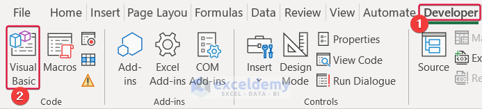
• Go to the Developer tab.
• From there, choose Visual Basic.

• In the Visual Basic window, choose ThisWorkbook under the VBAProject option.

• In the module, enter the following code and press Ctrl+S to save the code.

Private Sub PivotTableCache()
Dim am_pt As PivotTable
Dim am_ws As Worksheet
Dim am_pc As PivotCache
Application.ScreenUpdating = False
For Each am_ws In ActiveWorkbook.Worksheets
For Each am_pt In am_ws.PivotTables
am_pt.PivotCache.MissingItemsLimit = xlMissingItemsNone
Next am_pt
Next am_ws
For Each am_pc In ActiveWorkbook.PivotCaches
On Error Resume Next
am_pc.Refresh
Next am_pc
Application.ScreenUpdating = True
End Sub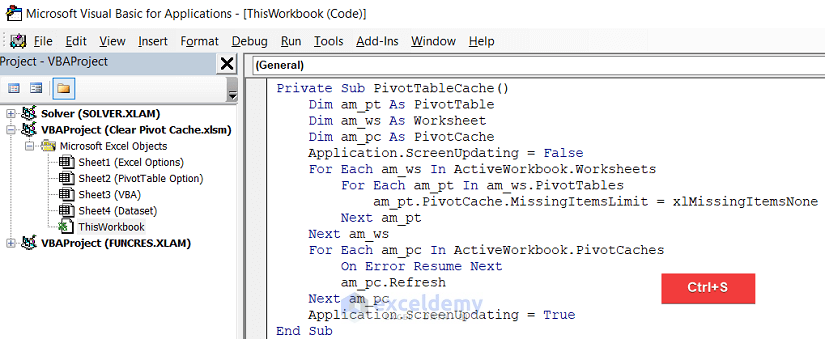

• Press F5 to run the code.

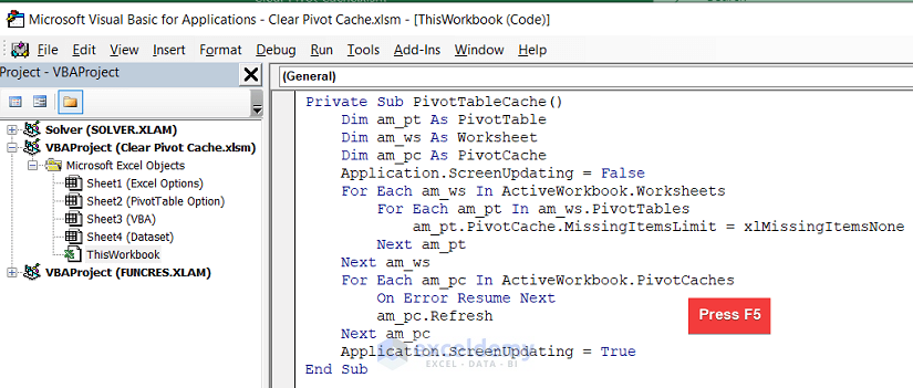
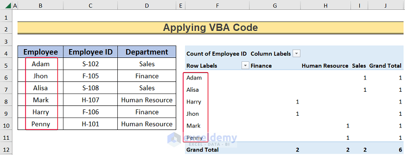
• The command will clear all the Pivot Cache and it will update the PivotTable.

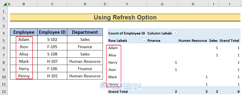
Method 3 – Using Refresh Command

Steps:

• Insert a PivotTable by using the data in the B5:D12 range like the first method.

• Select the B11:D12 cell range and right-click.
• From the options, choose Delete.

• In the pop-up box, select the Shift cells up option and click OK.

• The cells will be deleted from the data source.
• However, the data in the PivotTable will remain the same.

• Click on any of the data cells of the PivotTable and right-click.
• Choose Refresh from the available options.

• The command will terminate all the deleted data from the Pivot Cache.

Download Practice Workbook

<<Go Back to How to Delete Pivot Table | Pivot Table in Excel | Learn Excel