How to Summarize Data in Excel Using a Pivot Table (2 Methods)

Dataset Overview

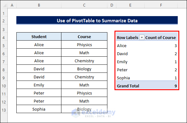
Let’s assume you have the below dataset containing duplicate values, and you want to quickly summarize it using a PivotTable.

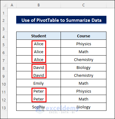
Method 1 – Using a PivotTable

Steps:

• Select the dataset or click anywhere within it.
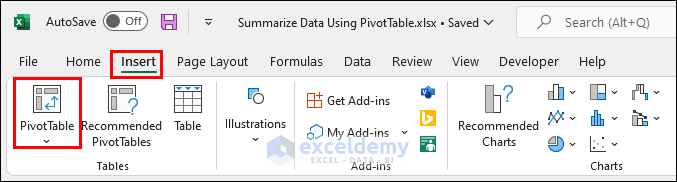
• Go to the Insert tab and choose PivotTable.

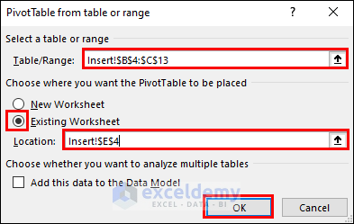
• Select the location where you want to place the PivotTable and click OK.

• Drag the relevant fields to the appropriate areas in the PivotTable Selection Pane.

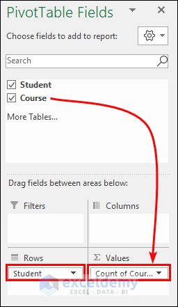
• The resulting PivotTable will display the count of courses taken by each student, eliminating the need to repeat their names.

Method 2 – Using DAX Functions

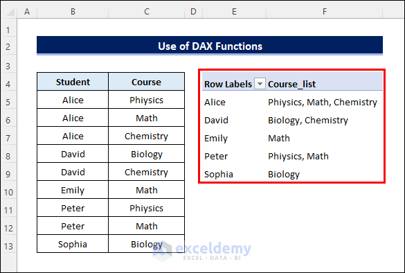
• Alternatively, you can concatenate the courses into a single cell within the PivotTable.
• Follow these steps

Steps:

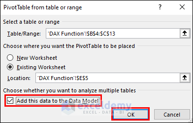
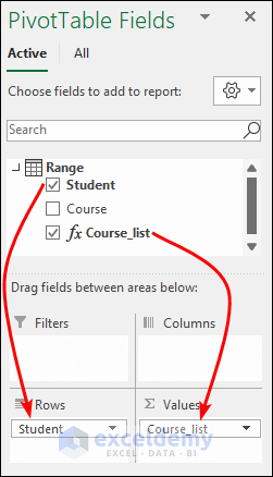
• While inserting the PivotTable, check the Add this data to the Data Model checkbox.

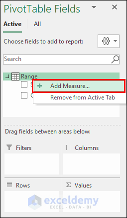
• Right-click on the Range field and select Add Measure.

• Enter a Measure Name (e.g., Course_list) and enter the following formula in the formula box:

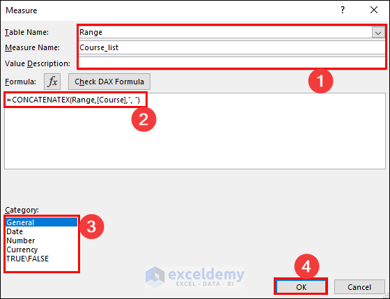
• Click OK.
• Drag the appropriate fields to the desired areas.

• You’ll achieve the desired result.

More PivotTable Features to Summarize Data in Excel

Here are some advanced PivotTable features to summarize data in Excel.

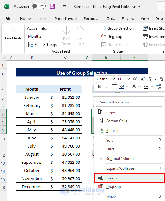
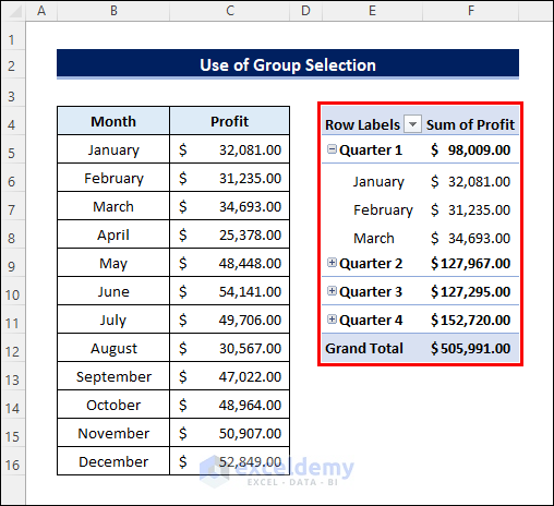
• Group Rows: Select specific rows in the PivotTable, right-click, and choose to group them.

• The summarized data will look as follows.

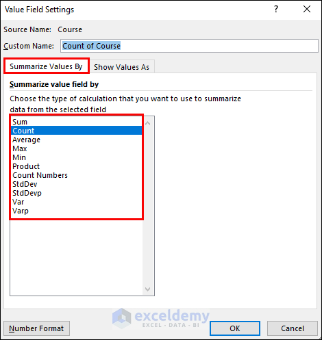
• Customize Summary Functions: Go to Value Field Settings and pick a different function to summarize the data.

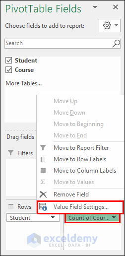
• Change the function as required from the Summarize Values By tab.

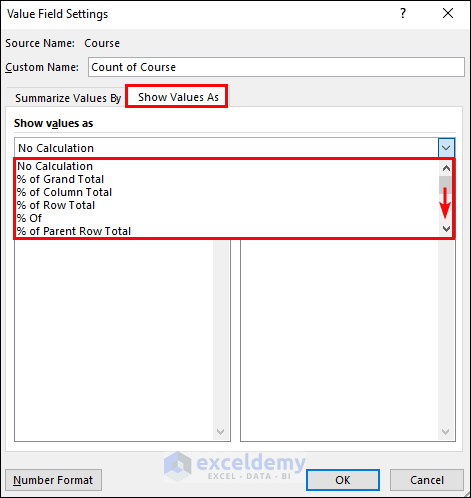
• Show Values Differently: Explore options in the Show Values As tab.

Things to Remember

• Always select anywhere in the PivotTable to access the editing tools.
• Drag fields to the appropriate areas until you achieve the desired result.

Download Practice Workbook

You can download the practice workbook from here:

Related Articles

• [Fixed!] Pivot Table Field Name Already Exists
• Pivot Table Field Name Is Not Valid
• Excel VBA to Get Pivot Table Field Names

<< Go Back to Pivot Table Field List | Pivot Table in Excel | Learn Excel