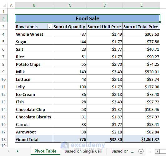
Suppose we have a Pivot Table dataset containing Products with their sold Quantity, Unit Price, and Total Price. We’ll format the pivot table.
Pivot Table Conditional Formatting Based on Another Column: 8 Easy Ways
Method 1 – Based on a Single Cell
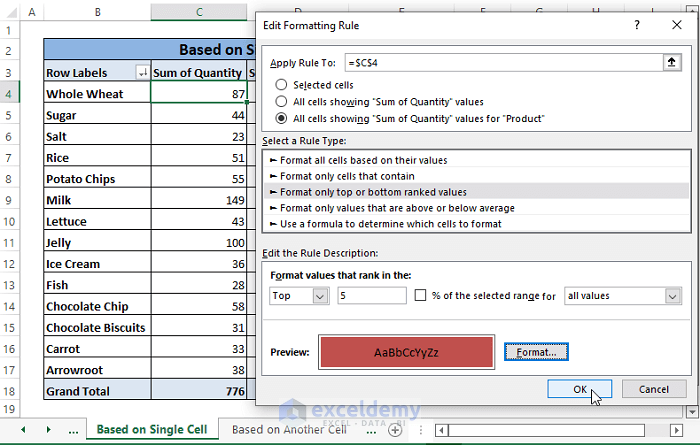
We want the top 5 Quantity values.
Steps:
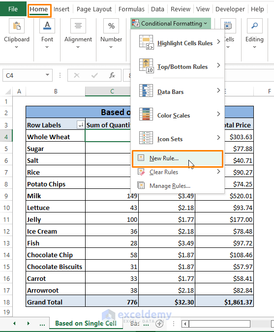
- Select any single cell in the column you want to format by (i.e., C4).
- Go to the Home tab and select Conditional Formatting (in the Styles section).
- Choose New Rule.
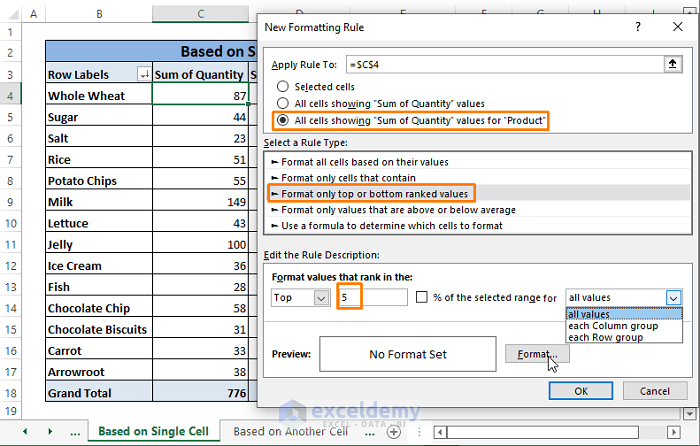
- A New Formatting Rule window opens up. Select the third option in the Apply Rule to and Select a Rule Type command box.
- Type 5 below the Edit Rule Description box. Keep the option all values within the last box in that row.
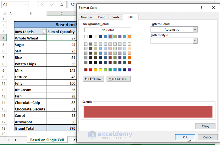
- Click on Format. The Format Cells window pops up.
- In the Format Cells window, choose any of the Fill colors.
- Click OK.
- Click OK.
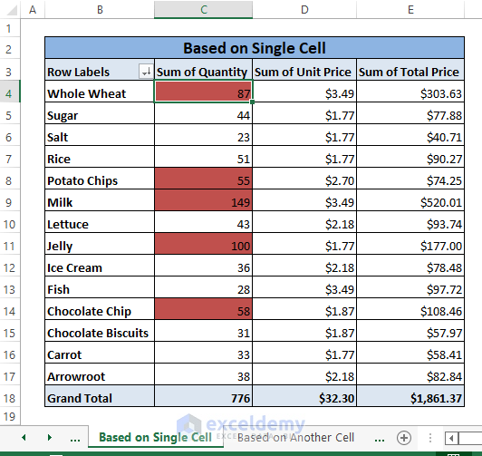
- This formats the top 5 cells in the Quantity column.
Method 2 – Based on Another Cell
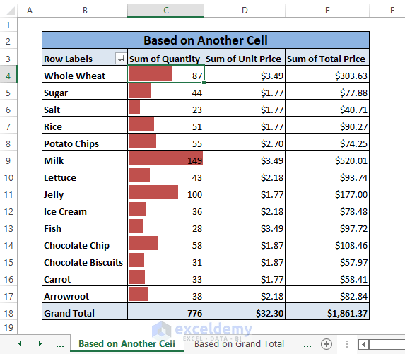
We have the sale Quantity of the Products and we want to compare them among the products to the most sold Product. In this case, Milk is the most sold product in the Pivot Table and we want to compare other products using the data bar.
Steps:
- Insert a New Formatting Rule.
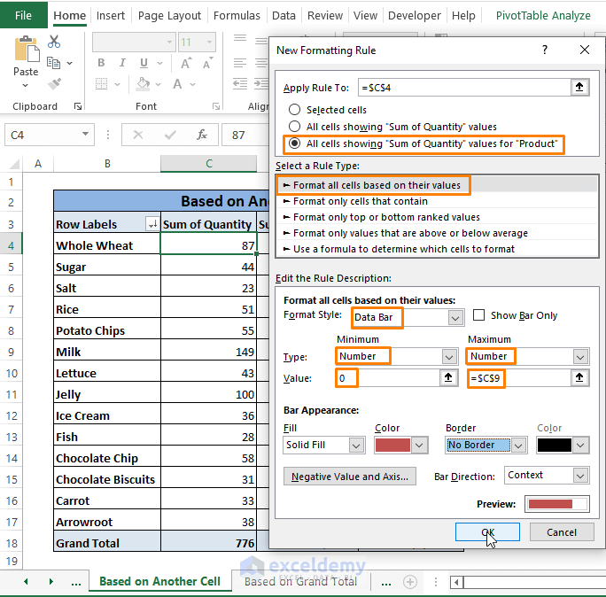
- In the New Formatting Rule window, select the 3rd and 1st options from Apply Rule to and Select a Rule Type command box, respectively.
- In the Edit the Rule Description dialog box, choose Data Bar as Format Style.
- Choose Number (both for Minimum and Maximum) for Type.
- Insert 0 as the Minimum value and Cell Reference C9 as the Maximum value (you can also input a formula to calculate the MAX of the range).
- Pick a Fill color then click OK.
- Here’s what you’ll get as the result, with partial bars to represent the sales against the maximum value.
Method 3 – Based on the Grand Total
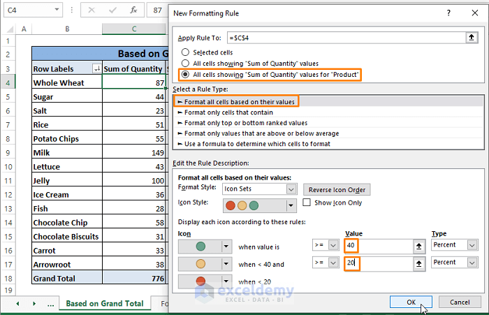
Let’s format the Quantity by their values. In this case, the highest value in the Quantity column is 149. We set Icon Sets to show 3-Color Icons for the representation of 40, 20, and below 20.
Steps:
- Create a New Formatting Rule.
- Inside the New Formatting Rule window, choose the 3rd and 1st options from Apply Rule to and Select a Rule Type command box, respectively.
- In the Edit the Rule Description dialog box, select Icon Sets as Format Style.
- In Display each icon according to these rules dialog box, insert 40 and 20 in Percent Type for Green and Yellow icons, respectively.
- Excel will automatically select the Red Icon Set for values less than 20 percent.
- Click OK.
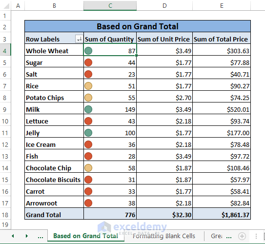
- The Icon Sets appear in the Pivot Table representing per percentage values they are set to refer to.
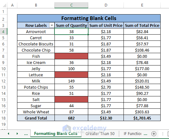
Method 4 – Based on Blank Cells
Let’s say we encounter zero sales for some products. We can conditionally format the entire Pivot Table depending on the blanks.
Steps:
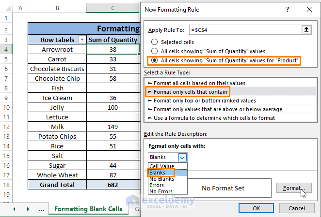
- Insert a New Formatting Rule.
- In the New Formatting Rule window, select the 3rd and 2nd options from Apply Rule to and Select a Rule Type command box, respectively.
- Inside the Edit the Rule Description dialog box, choose Blanks from Format only cells with a drop-down selection box.
- Click on Format.
- The Format Cells command window appears. Choose a Fill color.
- Click OK.
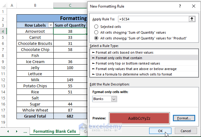
- All blank cells will be formatted.
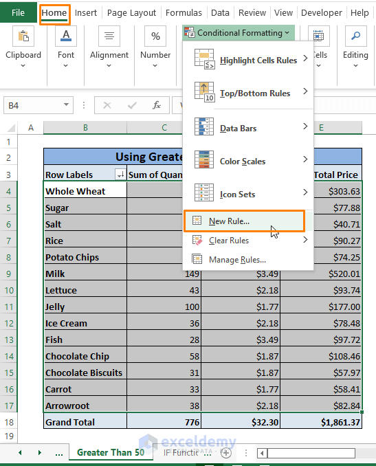
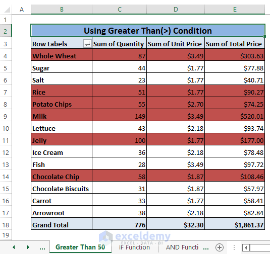
Method 5 – Using a Condition (Greater Than a Value)
We’ll format the rows that have sales Quantity greater than 50 (>50).
Steps:
- Select the entire Pivot Table (i.e., B4:E17).
- Go to Conditional Formatting and insert a New Rule.
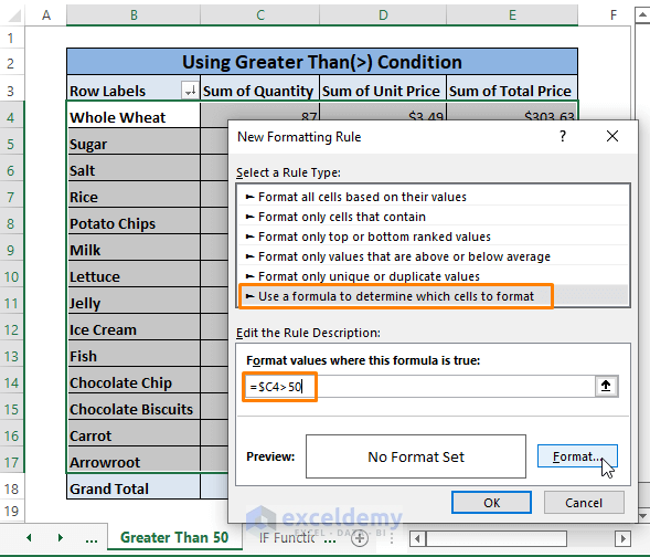
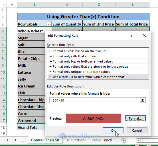
- This brings up the New Formatting Rule window. Select Use a formula to determine which cells to format.
- Inside the Edit the Rule Description command box, paste the following formula:
=$C4>50The Hashtag ($) before the Cell Reference (C4) ensures locking the Column Quantity (i.e., C column) to format the whole table based on the column.
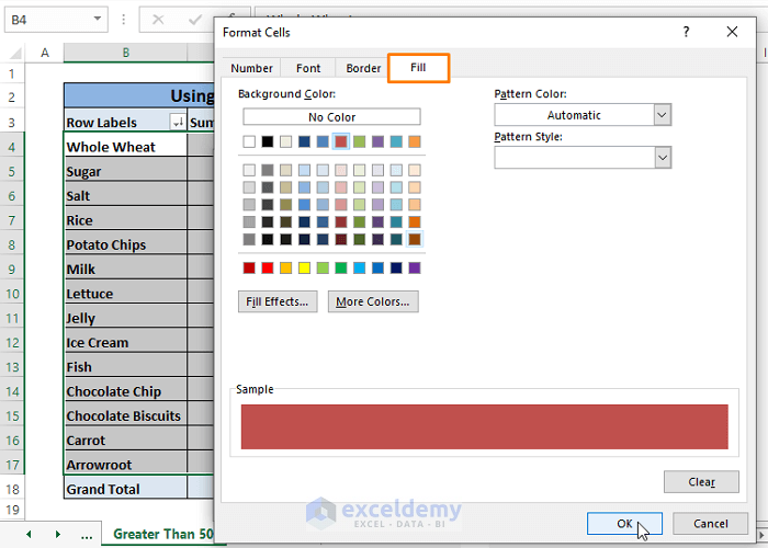
- Click on Format.
- From the Format Cells window, choose a Fill color, then click OK.
- After returning to the Formatting Rule window, click OK.
- Here’s the formatted table.
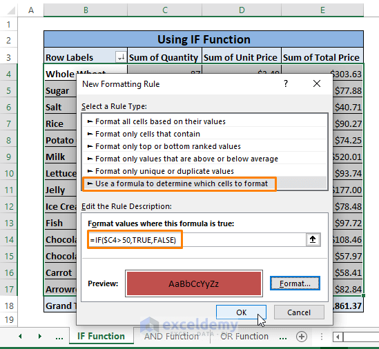
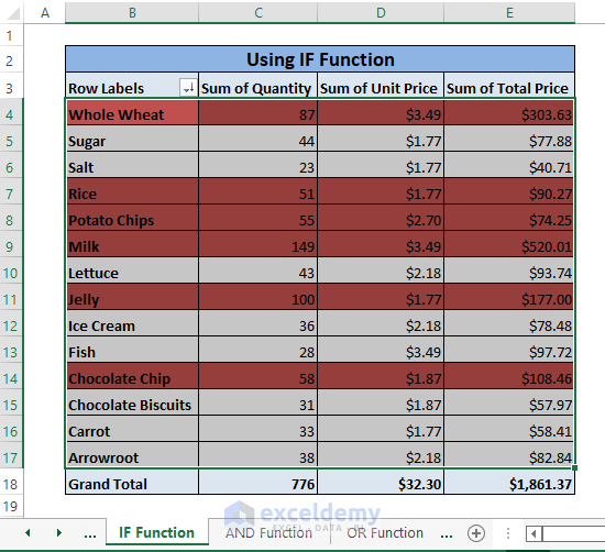
Method 6 – Using the IF Function
Steps:
- Follow the previous method, but replace the conditional formatting formula with the following:
=IF($C4>50, TRUE, FALSE)The IF function offers a logical_test ($C4>50) to conditionally format the entire Pivot Table based on the value in the row’s column C.
- Here’s the result.
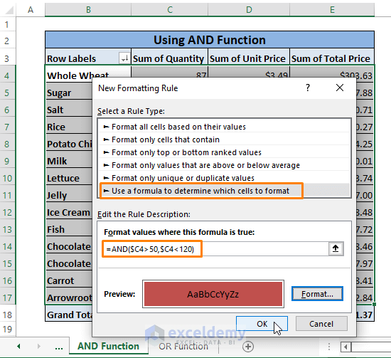
Method 7 – Using the AND Function
Let’s format quantities greater than 50 (>50) but lower than 120(<120).
Steps:
- Repeat Method 5, but replace the formula inside the Conditional Formatting New Rule with the following:
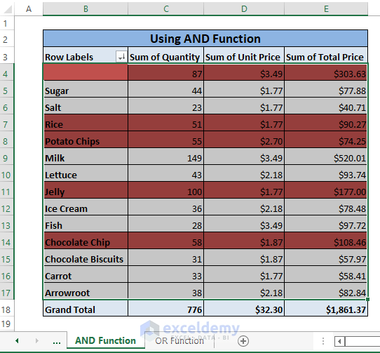
=AND($C4>50,$C4<120)The AND function offers two logical arguments as logical_tests ($C4>50,$C4<120). If both are true, it will output TRUE and Excel will format the cells.
- The formula formats all the rows that satisfy both of the arguments, similar to the image below.
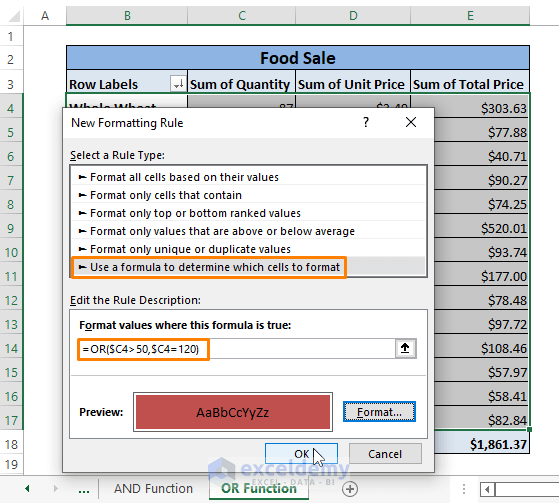
Method 8 – Using the OR Function
If you need only one of the conditions to be true, use the OR function.
Steps:
- Follow Method 5 and insert this formula for the formatting rule:
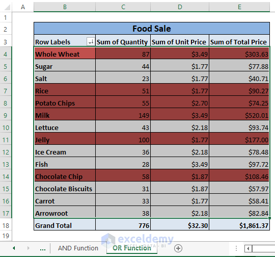
=OR($C4>50,$C4=120)The OR function checks whether $C4>50 or $C4=120 for Column C to format the whole Pivot Table.
- This results in the following image.
Dataset for Download

