Method 1. Using VBA to Highlight an Active Row in a Single Worksheet
Steps:
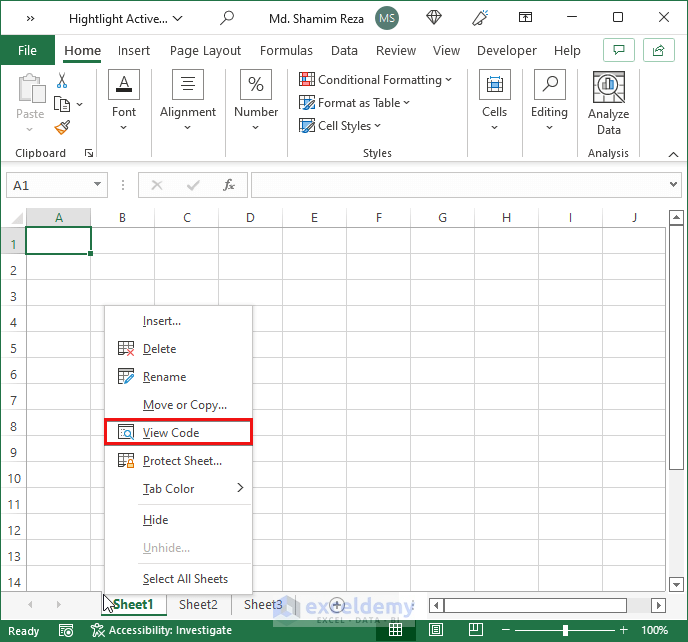
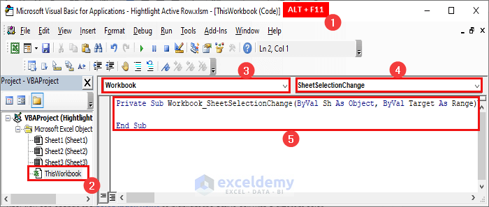
- Right-click on the sheet tab and select View Code. Alternatively, you can press ALT + F11 and double-click on the sheet name in the VB editor.
- Select Worksheet using the first dropdown in the code module. This will automatically insert a private subject procedure for the SelectionChange event.
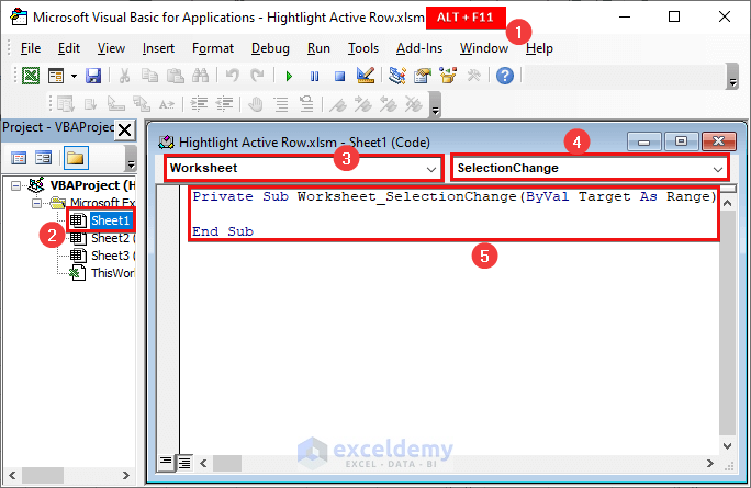
- Copy the following code and paste it inside the subject procedure.
Cells.Interior.ColorIndex = xlNone
With Selection
.EntireRow.Interior.ColorIndex = 40
End With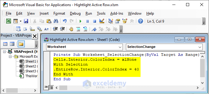
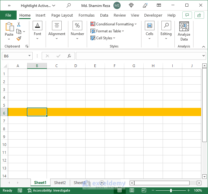
- Return to the worksheet and select any cell to see the result.
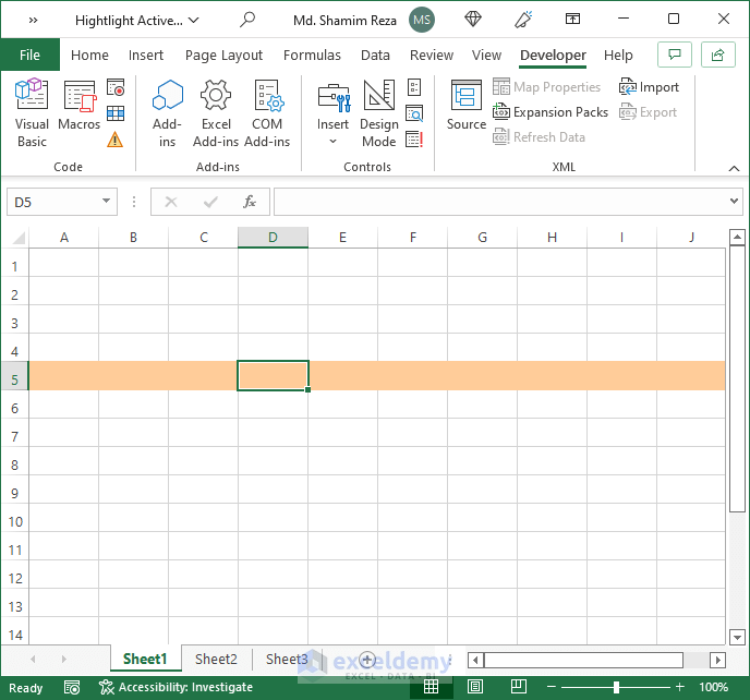
- It will highlight multiple rows. Just select cells from multiple rows to see the following result.
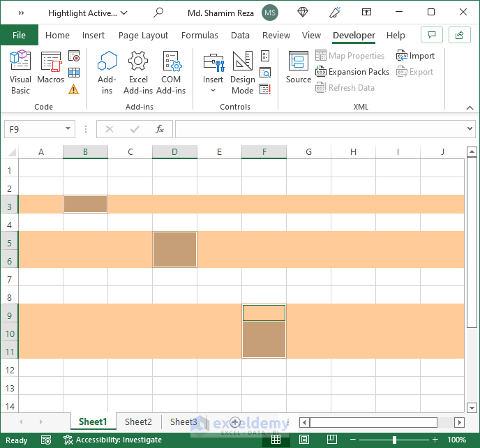
Tips: You can use the CTRL key to select non-adjacent cells or ranges.
- Copy the following code and paste it below the End With statement to highlight the active row except the selected cell.
Selection.Interior.ColorIndex = xlNone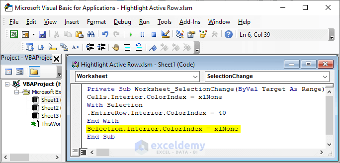
- The active row will be highlighted as follows.
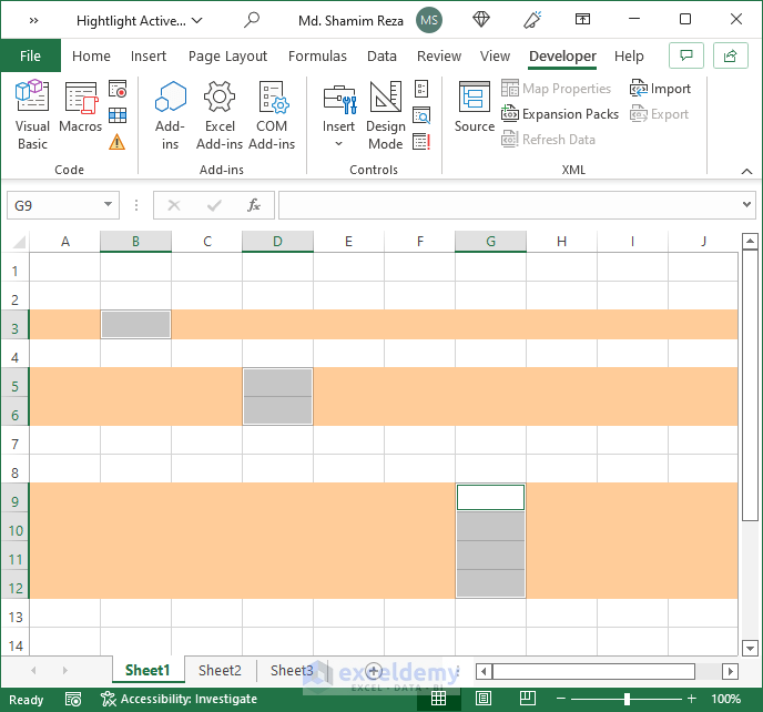
- You can add the following code before the End With statement to highlight the active column.
.EntireColumn.Interior.ColorIndex = 40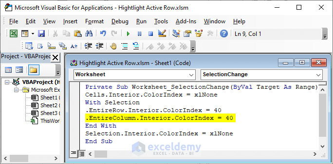
Tips:
You can change the color-index value to highlight the active cell with a different color. You can copy the code on each sheet to apply the highlighting effect in those worksheets.
Read More: How to Highlight Blank Cells in Excel VBA
Method 2 – Using VBA to Highlight an Active Row in an Entire Excel Workbook
Steps:
- Open the VB editor by pressing ALT + F11. You can also do it from the Developer tab.
- Double-click on This Workbook below the sheet names.
- Select Workbook and the SheetSelectionChange event using the dropdowns.
- A private subject procedure will be inserted for the event automatically.
- Delete all other procedures from that code module.
- Paste the same code used earlier inside this procedure.
Cells.Interior.ColorIndex = xlNone
With Selection
.EntireRow.Interior.ColorIndex = 40
End With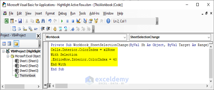
Whenever you go to a worksheet, the active row in that sheet will be highlighted automatically.
Read More: Excel VBA to Highlight Cell Based on Value
How to Highlight an Active Row in Excel without Using VBA Code
Steps:
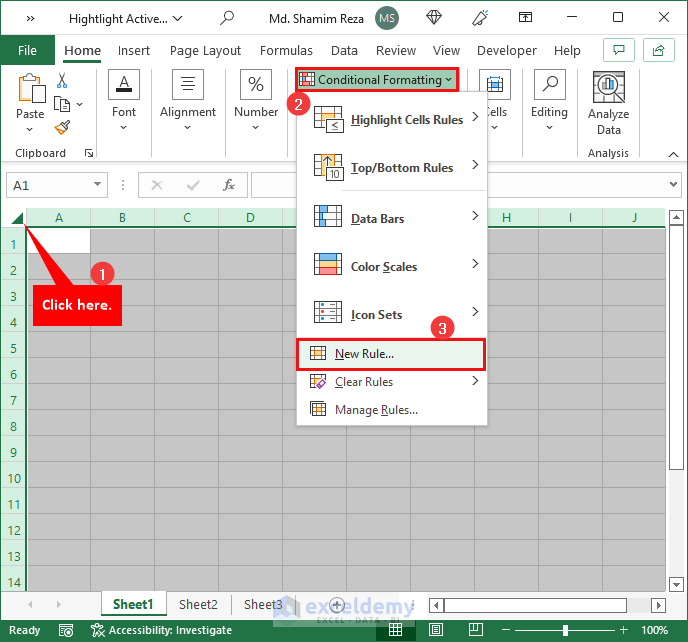
- Select the entire worksheet by clicking on the arrow at the upper left corner of the first cell.
- Select Home >> Conditional Formatting >> New Rule.
- The New Formatting Rule dialog box will appear.
- Select ‘Use a formula to determine which cells to format’ as the Rule Type.
- Enter the following formula in the formula box.
- Click on Format, pick a Fill Color, and click OK.
=CELL("ROW")=CELL("ROW",A1)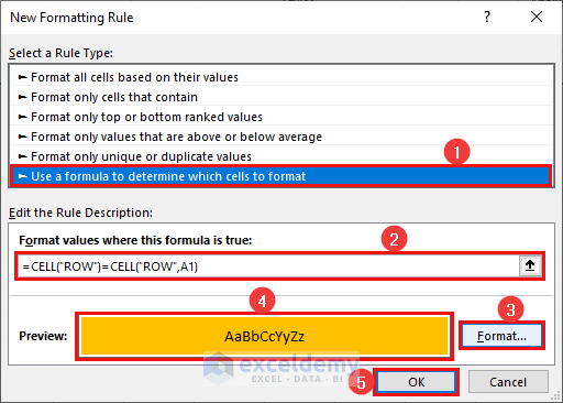
- Select any cell to see the active row highlighted as follows.
- Press F9 to refresh the selection when you click another cell. Otherwise, the earlier row will remain highlighted. You can also double-click and click away to refresh the worksheet.
- Using the following formula to highlight the active column, you can apply another conditional formatting.
=CELL("COL")=CELL("COL",A1)
Tips: You can press SHIFT + Space and CTRL + Space to highlight the active row and the active column temporarily.
Things to Remember
- Don’t forget to save the workbook as a macro-enabled workbook.
- You must copy the code to each sheet using the Worksheet SelectionChange event.
- You must insert the Workbook SheetSelectionChange event and copy the code to apply the highlighting effect to all worksheets.
- Change the color-index values in the code to apply different highlighting colors.
- While using conditional formatting, you must refresh the worksheet (press F9) to highlight the newly active row.
- It is better not to apply the worksheet and workbook events to the same sheet to highlight the active row.
Download the Practice Workbook
You can download the workbook to practice.

