Method 1 – Using Excel Power Query Editor to Consolidate Multiple Worksheets into One PivotTable
Steps:
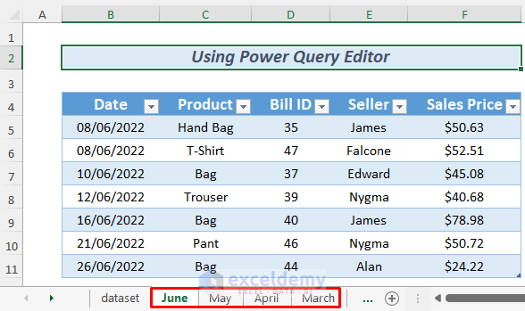
- Use the following sheets for consolidation into one Pivot Table.
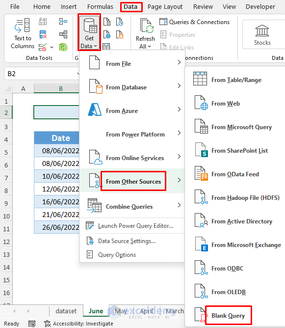
- Go to Data >> Get Data >> From Other Sources >> Blank Query.
- The Power Query Editor will open up.
- Give your Query a name. In my case, I named my query Overall_Report and hit ENTER.
- Type the following formula in the Power Query formula bar and hit ENTER.
=Excel.CurrentWorkbook()
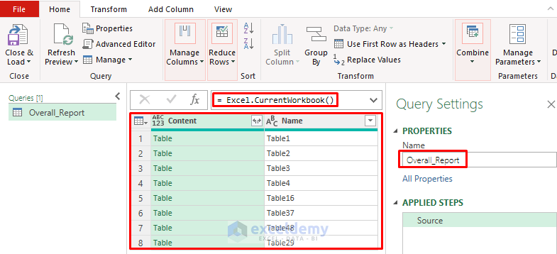
The formula will return all the tables in the workbook.
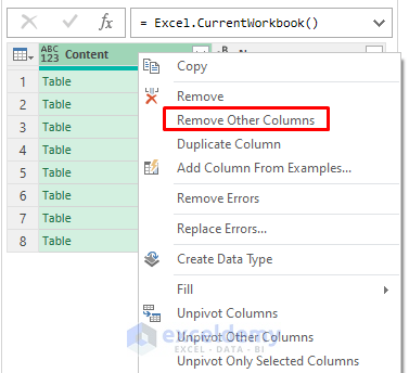
- We don’t need duplicates, we removed the second column using the Remove Other Columns command from the context menu, which we can get by right-clicking on the header of the first column.
- Select Home >> Keep Rows >> Keep Top Rows. We don’t need all the tables in this workbook.
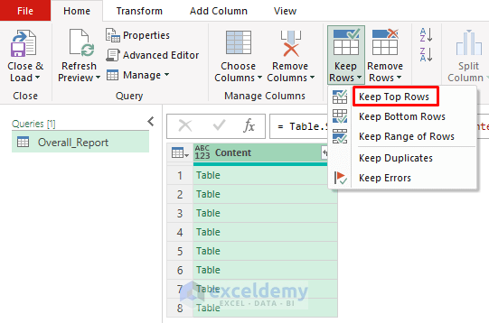
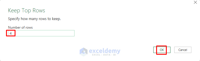
- The Keep Top Rows window will appear. As we are working with the first four tables of this workbook, we selected four.
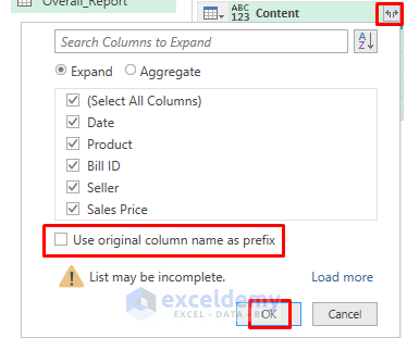
- This operation will return the first four rows only. Click on the marked icon of the following image, uncheck Use original column name as prefix and click OK.
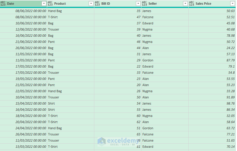
- See all the data of your sheets will consolidate together.
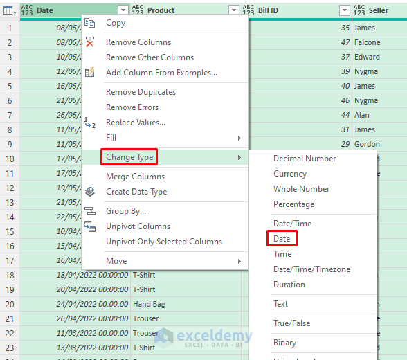
- The query may contain some unnecessary format like the date and time You will see there is a time after every date by default when the query opens. To remove this, we clicked right on the mouse while selecting the Date column and then chose Change Type >> Date.
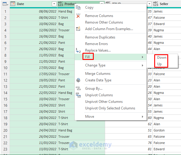
- If your data contains any blanks, use the following command. Select the columns that contain blanks and then right-click >> Fill. Select Down or Up according to your convenience.
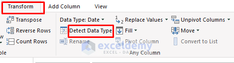
- Press CTRL+A and then go to Transform >> Detect Data Type. This command is not necessary all the but it’s a good practice while working with the Power Query Editor.
- Select Home >> Close & Load To…
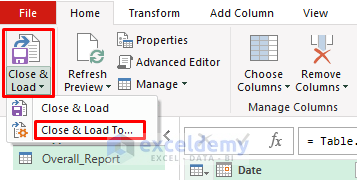
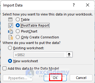
- The Import Data dialog box will appear. Select PivotTable Report, the sheet where you want the Pivot Table to be opened, and click OK.
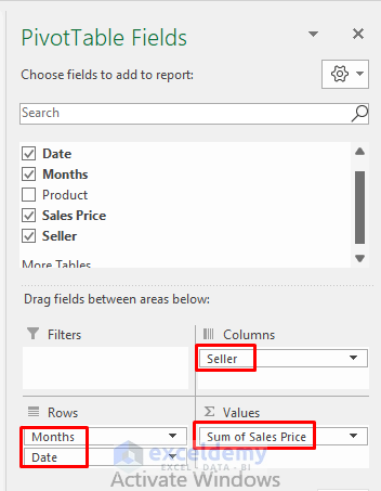
- See your Pivot Table in a new worksheet as we chose a New worksheet for it. Drag the Date range to the Rows Field, Sales Price to the Values Field, and Seller to the Columns Field to have a look at the summarized data of your worksheets.
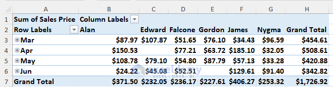
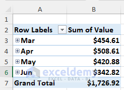
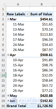
- See monthly and overall reports of the sales from March to June. You can also see seller based sales records in your Pivot Table.
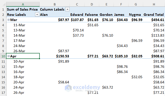
- Find more information about sales in a month, click on the Plus icon beside the month name. This will return you a date-based sales report.
Thus you can consolidate multiple worksheets into one Pivot Table by using a Power Query Editor.
Method 2 – Applying PivotTable and PivotChart Wizard to Consolidate Multiple Worksheets
Steps:
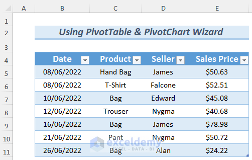
- We will be working with the Sales So we will use the same worksheets but we will omit the Bill ID column. It may cause some redundant calculations in the Pivot Table.
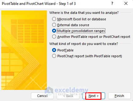
- Press ALT, D, and P You will see the PivotTable and PivotChart Wizard on the screen.
- Select the field where you want to analyze your data. As our article is dedicated to the Pivot Table, we select Multiple consolidation ranges and PivotTable. If you want to do a detailed analysis, you may select the PivotChart report instead of just PivotTable.
- Click Next.
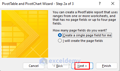
- You will have two options of how many page fields you require for analysis. You can either choose Excel to create a page field automatically for you, or you can make your own. Select Create a single page field for me which means Excel will create it automatically.
- Click Next.
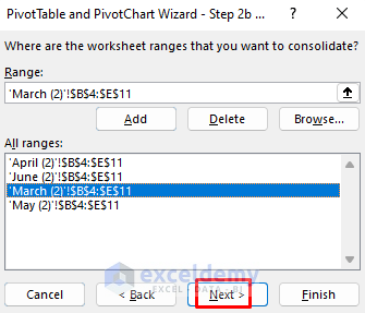
- See a message box where you will add the ranges of your tables for the Pivot Table Just select the sheet where the table of a sales report is, then select the table and click Add. We selected the table of June (2) sheet.
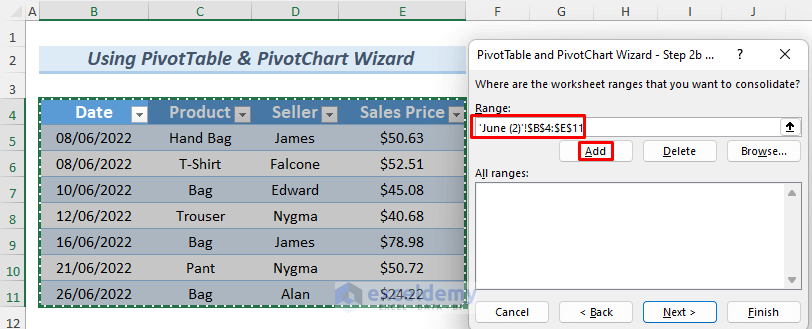
- Add the other tables too.
- Click Next.
- Select New worksheet or Existing worksheet based on your convenience.
- Click Finish after that.

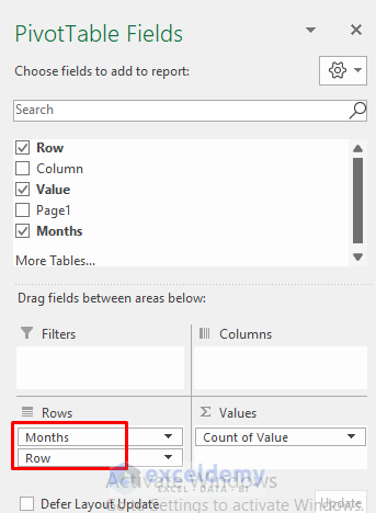
- This method is not as effective as the first one. We need to understand the meaning of the ranges in the PivotTable Fields. Here, Row refers to the dates and Value refers to the sales values. Drag Row and Value fields to the Rows and Values Fields
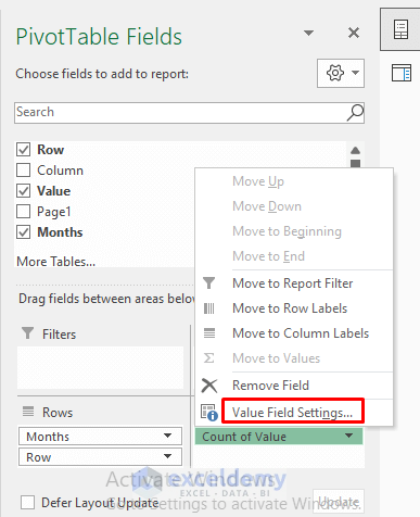
- Observe that the value field of the sales values is in Count of Value. We need the sales values and their total so we click on Count of Value field >> Value Field Settings.
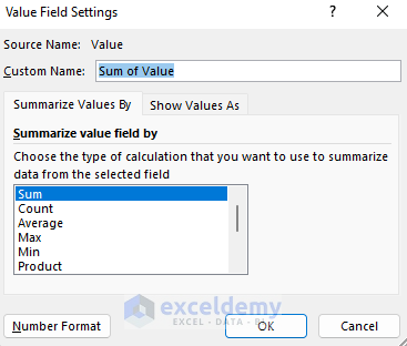
- In the Value Field Settings window, we select Sum of Value and click OK.
- This operation will return a monthly sales report in the Pivot Table.
- To expand your analysis on a daily basis, click the Plus icon beside the month name.
Thus you can consolidate multiple worksheets into one Pivot Table by using the PivotTable and PivotChart Wizard.
Download Practice Workbook

