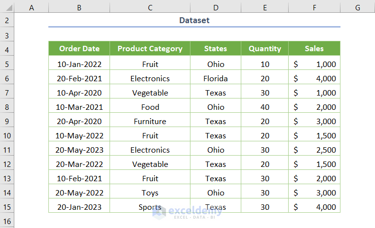
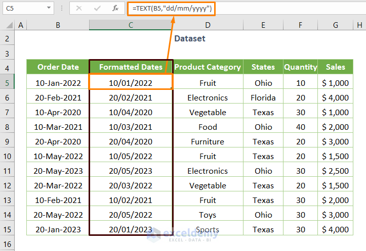
Let’s introduce today’s dataset where Sales of some Product Categories is provided along with an Order Date and corresponding States.
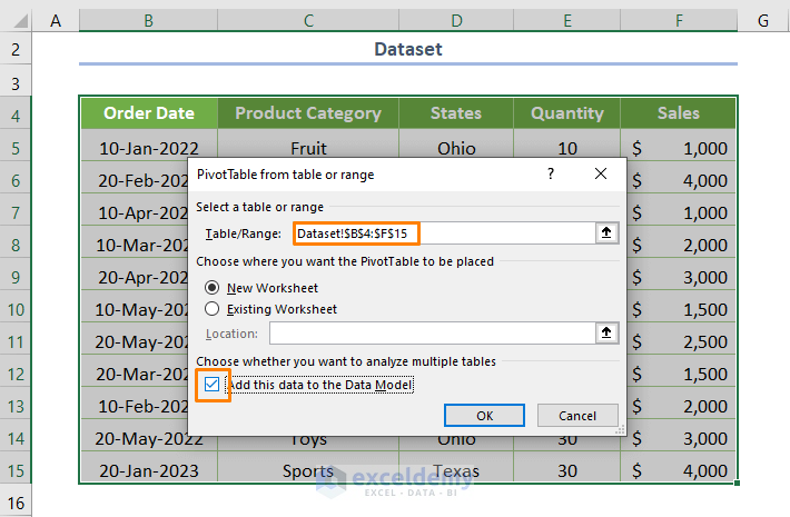
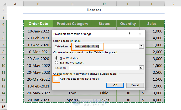
Creating a Pivot Table is a simple task. Check the circle before the New Worksheet and the box before the Add this data to the Data Model option.
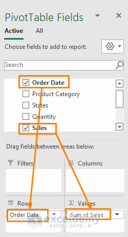
Move Order Date into the Rows area and Sales into the Values area.
You’ll get the following Pivot Table where the dates are automatically changed from the defined format in the source data. The date format in the source dataset is dd-mm-yyyy, but in the created Pivot Table it’s mm-dd-yyyy. Let’s see how you can change that.

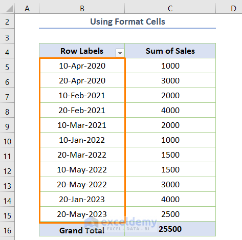
Method 1 – Using Format Cells to Change the Date Format in a Pivot Table
- Select the entire cell range first.
- Press Ctrl + 1 to open Format Cells.
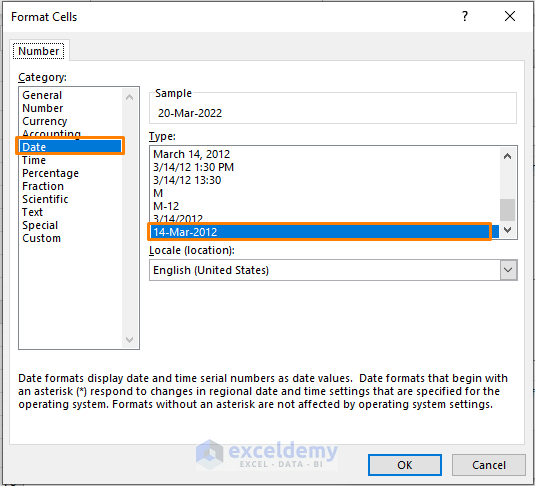
- Go to the Date category under the Number tab.
- Choose your desired date format (e.g. 14-Mar-2012).
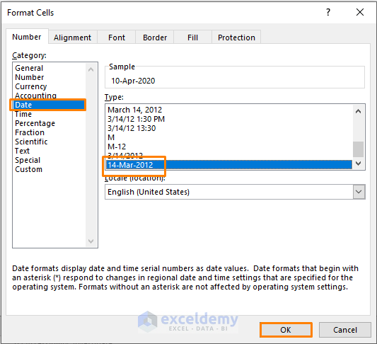
- Press OK.
- The dates will be changed and stored in your desired format as shown in the following screenshot.
Note: Using this simple method will be handy if you add your source data into the Data Model.
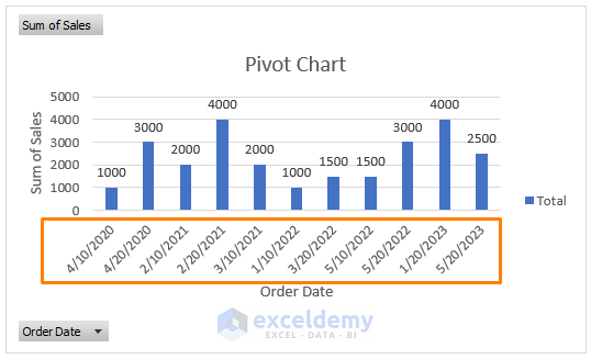
Method 2 – Changing the Date Format in a Pivot Table’s Chart
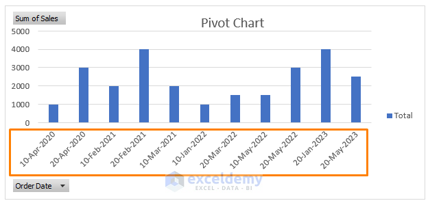
In the following example, we created a Pivot Chart from the previously generated Pivot Table. The date format is changed automatically in the horizontal axis of the chart.
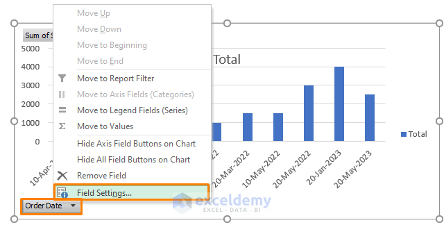
- Click on the Order Date box located at the lower-left corner of the chart.
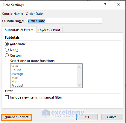
- Choose the Field Settings option.
- The dialog box of the Field Settings will open. Unfortunately, you won’t see the Number Format option at the lower-right side of the dialog box, because the Pivot Table is added to the Data Model.
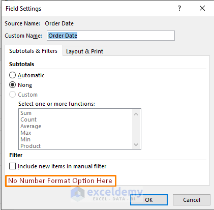
- To get the Number Format option, you need to uncheck the box for Add this data to the Data Model option when creating the Pivot Table.
- If you click on the Field Settings, you’ll get the Number Format option.
- Click on the option.
- You’ll get the as usual features of the Format Cells option.
- Choose your desired format and press OK.
- The Pivot Chart will change the dates in the horizontal axis.
Method 3 – Grouping Dates and Changing the Date Format in Pivot Table
Case 3.1 – Group Dates by Month
Let’s obtain the yearly summarized data.
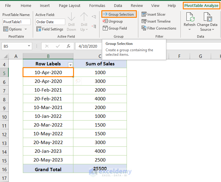
- Select a cell from the Order Date (Row Labels).
- Click on the Group Selection option in the PivotTable Analyze tab.
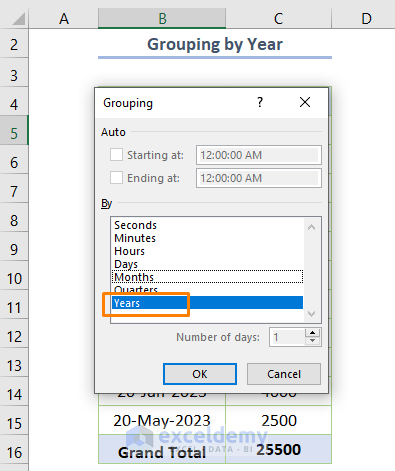
- You’ll get the following dialog box named Grouping. Choose Years from the options.
- Press OK.
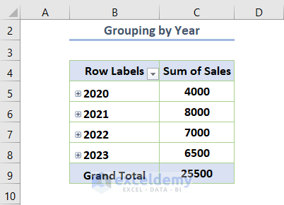
- You’ll get the yearly sums of sales.
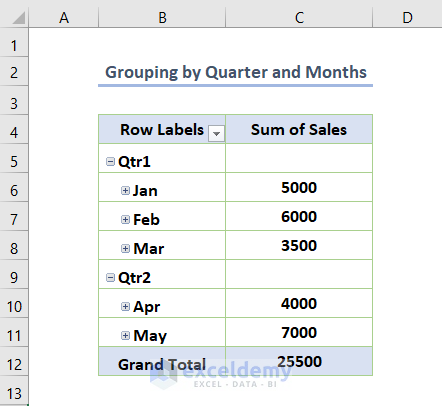
Case 3.2 – Grouping by Quarters and Months
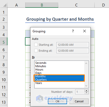
Let’s show the combined application of grouping by quarters and months.
- Follow the steps in the previous case and choose Months and Quarters in the Grouping dialog.
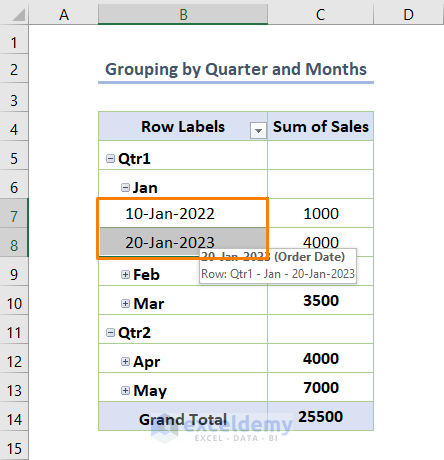
- The output will look like the following.
- If you click on the plus sign before the month name, you’ll get the dates. Then, you might use the Format Cells if you want to format the dates again.
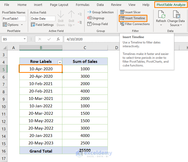
Case 3.3 – Inserting a Timeline Slicer
- Select a cell within the Order Date.
- Choose the Insert Timeline option from the Filter group in PivotTable Analyze.
- This type of timeline slicer typically sorts by year.
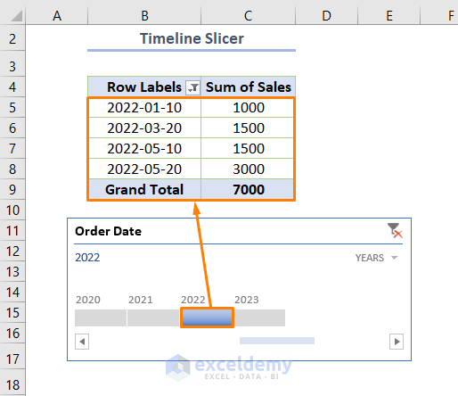
- Click on the gray-colored shape under 2022, and the timeline slicer shows all the sum of sales belonging to the year.
Method 4 – Ungrouping Dates and Adjusting Using Excel Functions
- Use the following formula in C5:
=TEXT(B5,”dd/mm/yyyy”)
Here, B5 is the starting cell of the Order Date and dd/mm/yyyy is the date format.
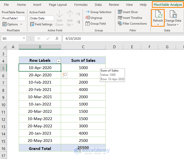
- Refresh the Pivot Table by clicking on the Refresh option in the PivotTable Analyze tab.
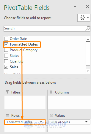
- Remove the previous Order Date field and add the Formatted Dates field in the Rows area.
- You’ll get your desired date format.
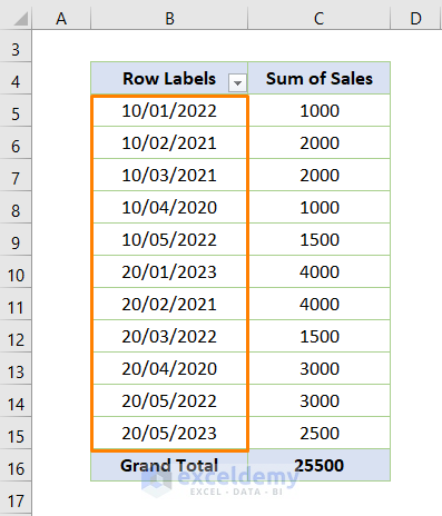
- You may change the date format into any valid format using the Excel function.
Read More: Remove Time from Date in Pivot Table in Excel
Things to Remember
While modifying the date format, you should be careful about the Data Model. For example, you may check whether the default option of turning on the Data Model for each Pivot table is checked or not.
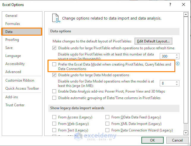
If you want to change the date format using the Number Format option from the Field Settings, make sure that you uncheck the box of the default option (yellow-colored in the following image). You can easily go to the Excel Options by clicking File and selecting Options.
Download Practice Workbook

