ikweethetnietmeer
New member
Dear all,
Please find the attachment.
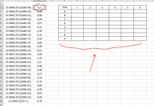
So, I have a list with 1 column sample names (A) and 1 column (B) their measured values.
Next to these columns I have a grid. I need to have the corresponding values in the exact place of the grid.
So far, I have been able to let Excel identify the text and put a value (in this case limited to B2) in the right position of the grid, but the only thing I cannot achieve is to have the correct measured value (in the corresponding adjecent cell) on that right spot in the grid in the right.
Please see the Excel sheet in the attachment and hope someone is able to help me out, this could save me a lot of data processing work.
Thanks a lot in advance!
Please find the attachment.
So, I have a list with 1 column sample names (A) and 1 column (B) their measured values.
Next to these columns I have a grid. I need to have the corresponding values in the exact place of the grid.
So far, I have been able to let Excel identify the text and put a value (in this case limited to B2) in the right position of the grid, but the only thing I cannot achieve is to have the correct measured value (in the corresponding adjecent cell) on that right spot in the grid in the right.
Please see the Excel sheet in the attachment and hope someone is able to help me out, this could save me a lot of data processing work.
Thanks a lot in advance!

") You helped me with saving a lot of time during my daily activities at work.
You helped me with saving a lot of time during my daily activities at work.