If you are searching for some special tricks to use slicer in Excel then you have landed in the right place. A Slicer is an interactive control. A Slicer makes your job easy to filter data in a pivot table. There are quick ways to create and use slicers in Excel. This article will show you each and every step with proper illustrations so, you can easily apply them for your purpose. Let’s get into the central part of the article.
Download Practice Workbook
You can download the practice workbook from here:
What Is Excel Slicer?
Slicer is an interactive way to Filter Excel Tables as well as Pivot Tables. It’s a smart way to Filter out data quickly. Along with filtering, the slicer shows the present criteria of filtering in an Excel Table or a Pivot Table.
Types of Excel Slicer
There are two types of Excel slicer:
- Pivot Table Slicer: It is used for filtering in the Pivot tables. For this, you have to create a pivot table first, then, from the PivotTable Fields window, you can create slicers.
- Table Slicer: It is possible to create slicers for Excel tables also. Through this, you can filter the table very easily.
3 Ways to Add Slicers in Excel
In this section, I will show you 3 quick and easy ways to add slicers in Excel on Windows operating system. You will find detailed explanations with clear illustrations of each thing in this article. I have used Microsoft 365 version here. But you can use any other versions as of your availability. If anything of this article doesn’t work in your version then leave us a comment.
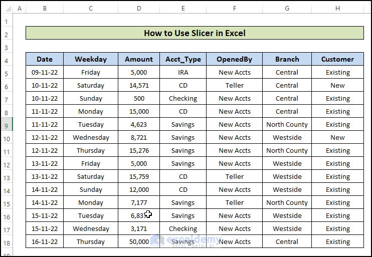
1. Use Slicer from Excel Pivot Table Fields
You can add a slicer from Excel PivotTable fields so you can easily filter by selecting items from the slicer. For this, follow the steps below.
Steps:
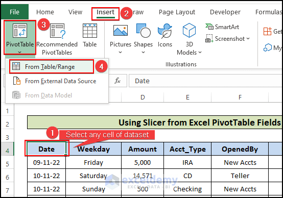
- First, you have to create a Pivot Table, for this select any cell from the dataset.
- Then, go to the Insert tab in the top ribbon.
- Here, click on the PivotTable menu and select the “From Table/Range” option.
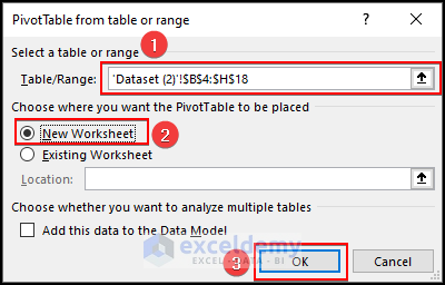
- Now, a pop-up window will appear.
- Here, the range of the dataset will be selected automatically in the Table/Range
- Select the New Worksheet
- Then, press OK.
- Now, a new worksheet will create where the pivot table is stored. Click on the pivot table and you will see a PivotTable Fields window will appear on the right side of the worksheet.
- Now, mark the items and drag them to rows and columns to create a pivot table.
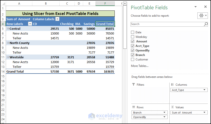
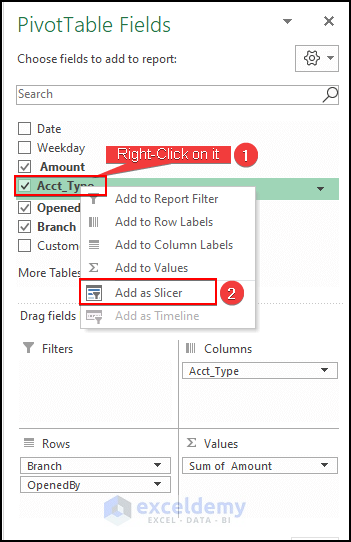
- In the Pivot Table window, right-click on an item and you find an option named “Add as Slicer”.
- Click on it to create a slicer for that item.
- As a result, in the Excel worksheet, you see a slicer Drag and move it to a suitable position.
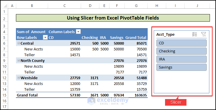
- Thus, the slicer is created and you can filter the dataset by account types using the slicer.
Read More: Excel Slicer for Multiple Pivot Tables (Connection and Usage)
2. Insert Slicer from Pivot Table Analyze Tab
We can use also the PivotTable Analyze tab to create a slicer for any pivot table. For this, you have to create a pivot table first for the dataset. You can follow the steps shown previous method to create a pivot table. And to create a slicer using the Pivot table Analyze tab, follow the steps below.
Steps:
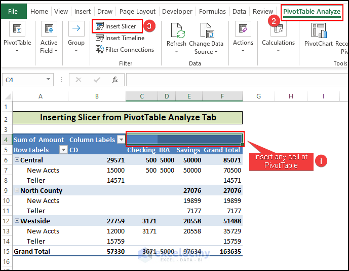
- First, select any cell of the pivot table.
- Then, you will see a new tab will be created in the top ribbon named “PivotTable Analyze”. Go to this tab.
- Here, you find the “Insert Slicer” option in the Filter Go to this option.
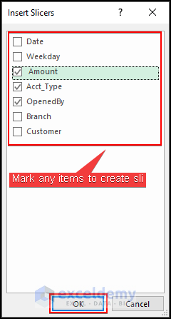
- Then, a new pop-up window will appear named “Insert Slicer”.
- Here, you will see the name of the column headers name as a list.
- Mark the options as you want to create slicers.
- Then, press OK.
- As a result, you will see that for the selected column headers, slicers will create.
- Click on the top right corner of the slicer to select it. Then, drag or move the slicer to a suitable position.
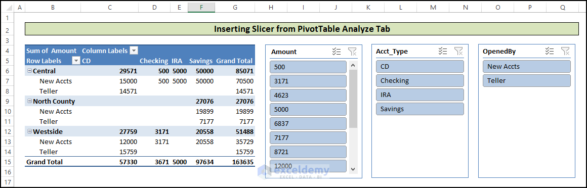
- Thus, you have created slicers for the pivot table from the Analyze tab.
Read More: How to Insert Slicer in Excel (3 Simple Methods)
3. Insert Slicer to Excel Table from Design Tab
You can also create slicers also for any Excel tables. So, for this, you have to convert the dataset to an Excel table then you can create slicers for the table to filter data accordingly. Follow the steps below.
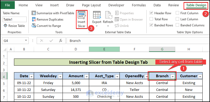
Steps:
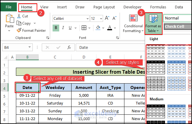
- To convert the dataset into an Excel table, select any cell of the dataset.
- Then, go to the Home tab and click on the “Format as Table” option.
- Then, a list of styles will appear and select any of them to apply.
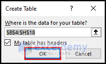
- Now, a pop-up window named “Create Table” will appear.
- Here, you will see that the range of the dataset is already selected in the box.
- Mark the box saying “My table has headers”.
- Then, press OK.
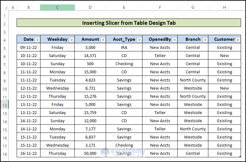
- As a result, you will see that the dataset is converted into a table. And there will create a filter arrow in each column header.
- Now, click on any cell of the excel table.
- After that, there will create a new tab named “Table Design” on the top ribbon.
- Here, click on the “Insert Slicer” option under this tab.
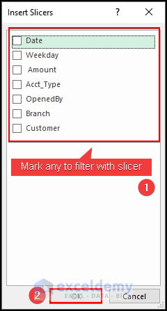
- Then, another new pop-up window will appear named “Insert Slicers”.
- Mark the items for which you want to create slicers.
- Then, press OK.
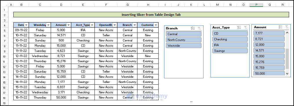
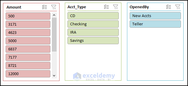
- Now, you will see that there will create slicers for the selected items. Now, you can easily filter the data table using the slicers. Thus, you can create an Excel dashboard with slicers.
Read More: How to Insert Slicer without Pivot Table in Excel
Use of Excel Slicers
You can use slicers for various purposes in Excel. The main purpose of the slicer is to filter an Excel table and Pivot Table easily. Follow the steps below to use Slicers for any tables or Pivot tables.
- After creating slicers, you can choose any of the items from the slicer to filter the table.
- Then, click on the item to show the dataset only for that item. Like here, I have created a slicer of Branch. So, when I select the item “Central” in the slicer then the dataset is automatically filtered for the central branch.
- You can select multiple items in the slicers. For this, you have to hold the Ctrl key on the keyboard and select the items one by one from the slicer.
- Similarly, you can filter for any other items from the slicer.
How to Format to Create Fancy Slicers in Excel
You can change the formatting of the slicers created in Microsoft Excel. Here, I am showing you how you can format the slicers to look more attractive. Follow the steps below.
Steps:
- First, you have to select the slicer.
- Then, you will see that there will create a new tab named Slicer on the top ribbon.
- Under the Slicer tab, you will find many styles which you can apply to the slicer.
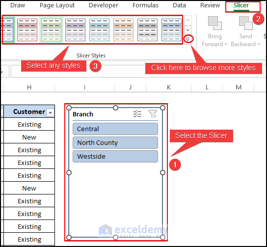
- Change the style of the slicers and it will look fancier.
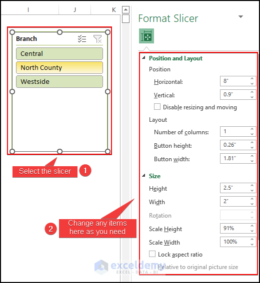
- Also, you can change other formatting options. When you select the slicer then, you will see a new window on the right side of the worksheet named “Format Slicer”.
- Here, you can change the Position, height, width, and some things of the slicer.
- Most importantly, you can convert the slicer into two or more columns. You can change the column number from the “Number of Columns” under the Layout menu here.
Conclusion
In this article, you have found how to use slicers in Excel. I hope you found this article helpful. You can visit our website ExcelDemy to learn more Excel-related content. Please, drop comments, suggestions, or queries if you have any in the comment section below.
Related Articles
- How to Resize a Slicer in Excel (With Quick Steps)
- Connect Slicer to Multiple Pivot Tables from Different Data Source
- [Fixed] Report Connections Slicer Not Showing All Pivot Tables

