Performing a comparison between a couple of lists is one of the familiar tasks in Excel. Today we will show how to compare two lists using the VLOOKUP function with 2 ideal examples.
VLOOKUP to Compare Two Lists in Excel: 2 Ideal Examples
Here we have a dataset of equipment lists of two gyms. We will compare the lists using the VLOOKUP function with 2 ideal examples.
Note that this is a basic dataset with dummy data. In a real-life scenario, you may encounter a much larger and more complex dataset.
1. Compare Two Lists in Same Sheet Using VLOOKUP Function in Excel
In this section, we are going to see how to compare two lists when they are within the same worksheet. For example, we will compare whether the equipment from Gym 2 is present within the Gym 1 equipment list or not.
STEP 1: Insert Simple VLOOKUP Formula
It’s obvious that our working formula consists of the VLOOKUP function. Follow the procedures given below.
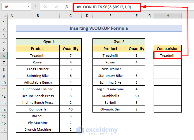
- First, write the following formula in Cell H6.
=VLOOKUP(E6,$B$6:$B$17,1,0)- Press Enter.
In the formula,
- we have set the element from Gym 2 as lookup_value and the equipment from Gym 1 as lookup_array. And this will return the equipment name when it is found within the Gym 1box.
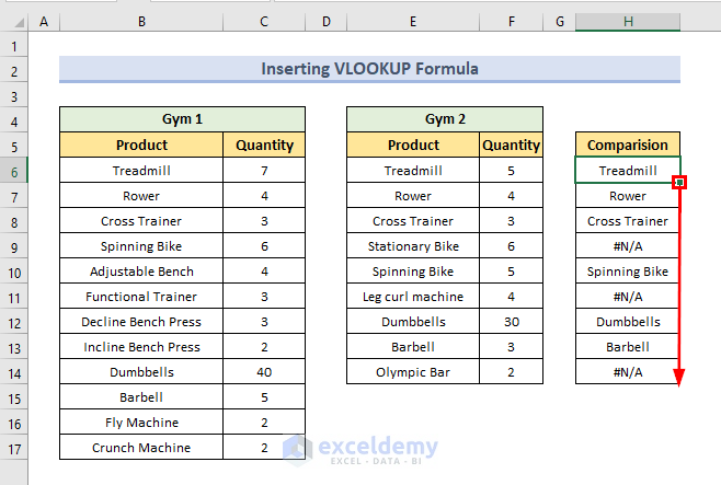
- Finally, use the Fill Handle to copy the formula in the cells below.
- Consecutively, we will see the result in every cell.
STEP 2: Use ISNA Function for Error Handling
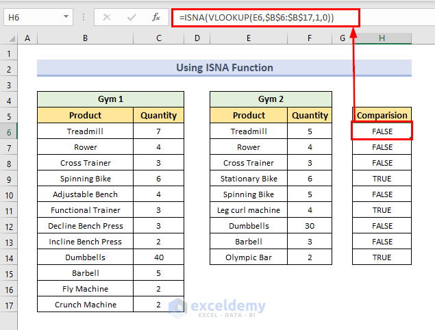
A clean sheet hardly contains any errors. So we should rectify the error. Now, we need to rewrite the formula in such a way that it doesn’t return an error for a value that is not present within the comparing list. For this, we are going to use the ISNA function. ISNA checks whether a value is #N/A, and returns TRUE or FALSE. To know about the function, visit this ISNA article. Follow the procedure given below for this step.
- First, write the following formula in Cell H6.
=ISNA(VLOOKUP(E6,$B$6:$B$17,1,0))- Next, press Enter.
- Further, use the Fill Handle to copy the formula in the following cells.
- Instantly, we will see the result in every cell as True or False.
STEP 3: Apply Additional NOT Function to Clarify
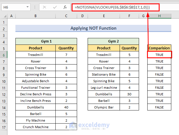
Sometimes, it might be confusing when you get FALSE for a value that is present within the list and TRUE for a value that is not in the list. To get rid of this kind of issue, we can use the NOT function. The NOT function gets the opposite of a specified logical or Boolean value. When you insert TRUE, it shows FALSE. When you insert FALSE, it shows TRUE. Let’s follow the steps given below for the procedures.
- Write the following formula in Cell H6.
=NOT(ISNA(VLOOKUP(E6,$B$6:$B$17,1,0)))- Consecutively, press Enter and use the Fill Handle to copy the formula in the following cells.
- Simultaneously, we will see True or False like the picture below.
- This will return TRUE when the item is found within the list and for comparing a value that is not within the list the formula will return FALSE.
STEP 4: Insert IF Function for Making Things User Friendly
Mere TRUE and FALSE may not be a reader-friendly description. If you open the file a few days later or a new reader goes through the file then there may be some confusion. To make things easily understandable we can use the IF function. Follow the steps given below for the procedures.
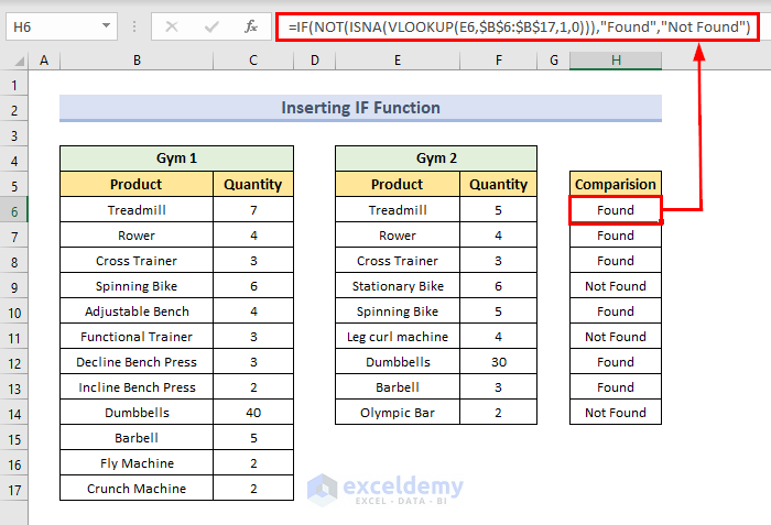
- First, write the following formula in Cell H6 and press Enter.
=IF(NOT(ISNA(VLOOKUP(E6,$B$6:$B$17,1,0))),"Found","Not Found")- Later on, use the Fill Handle to copy the formula in the following cells.
- Simultaneously, we will see Found or Not Found in every cell.
In the formula,
- In the condition check field of IF, we have inserted the previously used NOT-ISNA-VLOOKUP formula.
- We have set “Found” and “Not Found” as the if_true_value and if_false_value respectively.
- When the condition is TRUE (equipment is in the list) the formula will return “Found”.
- And when the condition is FALSE (equipment is not in the list) the formula will return “Not Found”.
2. Compare Two Lists in Different Sheets Using VLOOKUP Function in Excel
The lists can be located on two different sheets like here. Here, we have Gym 1 equipment in the Gym 1 sheet.
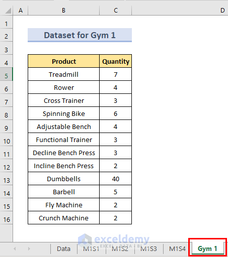
And in another M2 sheet, we have the item for Gym 2. We will compare the values in the M2 sheet. Follow the steps given below for the procedures.
- First, open the active sheet where we will do the comparison.
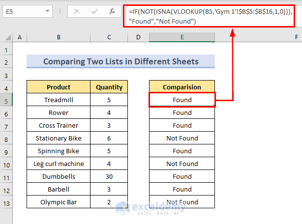
- In Cell E5, write the following formula.
=IF(NOT(ISNA(VLOOKUP(B5,'Gym 1'!$B$5:$B$16,1,0))),"Found","Not Found")- Then, press Enter and use the Fill Handle to copy the formula in the following cells.
- Simultaneously, we will see the comparison result for every item.
Note:
- We are comparing in the M2 sheet, so we need to provide this sheet name, but the lookup_array value is in the separate sheet Gym 1. That is we need to provide the sheet name so that, Excel can understand where to find it.
- After providing the sheet name make sure to insert an exclamatory sign (!). And if the sheet name has multiple words then put the name within a single quote (”).
Read More: VLOOKUP Example Between Two Sheets in Excel
A Suitable Alternative of Using VLOOKUP for Comparing Two Lists in Excel
In Excel, you can perform a single task in various ways. This comparison task is also not beyond that. Here is an honorable mention that you can use as an alternative to VLOOKUP.
Instead of VLOOKUP, we can use the COUNTIF function. Follow the steps given below for the procedures.
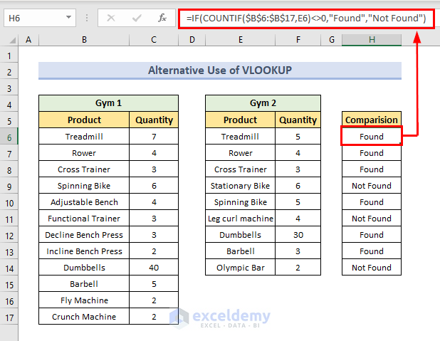
- Firstly, write the following formula in Cell H6.
=IF(COUNTIF($B$6:$B$17,E6)<>0,"Found","Not Found")- After that, press Enter and use the Fill Handle to copy the formula in the following cells.
- Finally, we will see the comparison result for every item.
In the formula,
- Within the COUNTIF we have checked whether occurrences of the lookup value are not equal to 0 or not.
- If not 0 (means the product presents in the list), then it returns “Found”, otherwise “Not Found”.
Download Practice Workbook
You can download the practice workbook from here.
Conclusion
That’s all for today. We have shown how to use VLOOKUP to compare two lists. Hope you will find this helpful. Feel free to comment if anything seems difficult to understand. Let us know any other approaches that we might have missed here.
Further Readings
- How to Use VLOOKUP for Multiple Columns in Excel
- VLOOKUP from Multiple Columns with Only One Return in Excel
- How to Use VLOOKUP to Return Multiple Columns in Excel
- How to Use the VLOOKUP Ascending Order in Excel
- VLOOKUP with Drop Down List in Excel
- How to Use VLOOKUP for Rows in Excel
- How to Use Column Index Number Effectively in Excel VLOOKUP
- Perform VLOOKUP by Using Column Index Number from Another Sheet
- How to Find Column Index Number in Excel VLOOKUP
<< Go Back to VLOOKUP a Range | Excel VLOOKUP Function | Excel Functions | Learn Excel
Get FREE Advanced Excel Exercises with Solutions!
