Transposing data in Microsoft Excel is truly one of the most common tasks performed by Excel users. Indeed, there are many ways for transposing row to column in Excel. In this article, we will demonstrate 6 easy and effective methods with proper explanations and illustrations to transpose rows to columns in Excel. So, go through the entire article to understand the topic properly.
Download Practice Workbook
You may download the following Excel workbook for better understanding and practice.
6 Methods to Transpose Rows to Columns in Excel
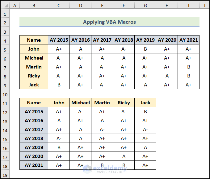
Assuming that we have a data set that presents the year-wise Results of Students. This dataset includes the Names and consecutive year-wise results under column B to column I.
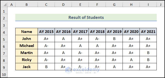
Now, we want to transpose the rows of this data set to columns for the sake of better presentation. In the following sections, we will show 6 instrumental Excel methods to perform this task. So, let’s explore them one by one.
Here, we have used the Microsoft Excel 365 version, you may use any other version according to your convenience. Please leave a comment if any part of this article does not work in your version.
1. Using Paste Special Command
We can use the simple Paste Special command in two ways, as described below.
1.1 Paste Special Command from Ribbon
This method is quick and easy, but it’s not suited for repeated processes. However, let’s see how this method works.
📌 Steps:
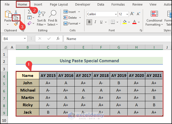
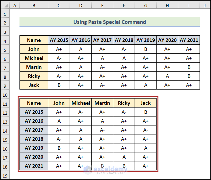
- First of all, select cells in the B4:I9 range that you want to transpose.
- Then, navigate to the Home tab.
- After that, click on the Copy icon on the Clipboard group of commands.
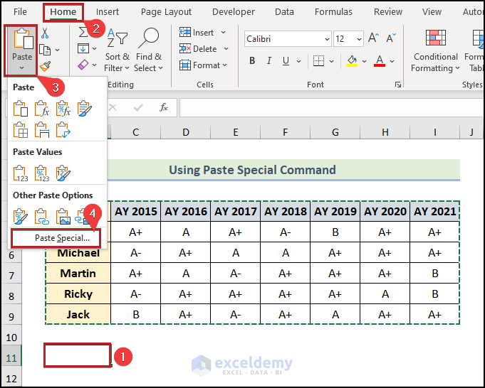
- Afterward, choose cell B11 where you finally want the output.
- Next, go to the Home tab.
- Later, click on the Paste drop-down icon on the Clipboard group.
- Hereafter, select Paste Special from the drop-down list.
Immediately, the Paste Special dialog box will pop up.
- Here, check the box of Transpose.
- Lastly, click OK.
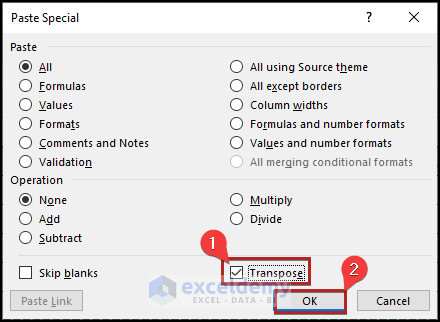
As a result, you can see the new output in the B11:G18 range which is the transposed form of the dataset. Notice that the rows get the places of the columns.
1.2 From Keyboard Shortcut
Wouldn’t it be great if there were keyboard shortcuts to do the same task? Well, you’re in luck, because it exists. It’s simple and easy; just follow along.
📌 Steps:
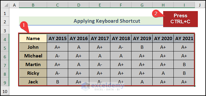
- Later, select cell B11 as the first cell of the destination range.
- Next, press CTRL + ALT + V keys on the keyboard.
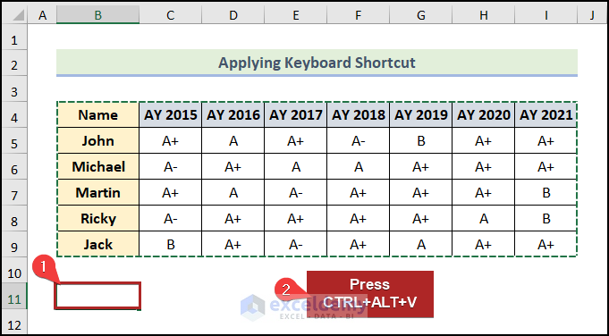
Consequently, the Paste Special dialog box will open.
- Then, press E to check the box of Transpose.
- Following this, click OK or press ENTER.
![]()
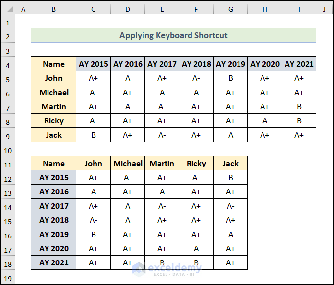
Finally, you got the transposed result.
Read More: How to Paste Transpose in Excel Using Shortcut (4 Easy Ways)
2. Transposing a Table and Linking It to Initial Data
A drawback of Method 1 above is due to a change in any data in the initial data set, it won’t change in the transposed data set. So, we need a method that’ll link up the output with the initial data set and will update accordingly. Following the steps below, let’s see how to do this.
📌 Steps:
- At first, select cells in the B4:I9 range.
- Secondly, press CTRL + C on the keyboard.
- Thirdly, select cell B11 where you want to place the output.
- Then, press CTRL + ALT + V on your keyboard.
- After that, click on the Paste Link on the Paste Special wizard.
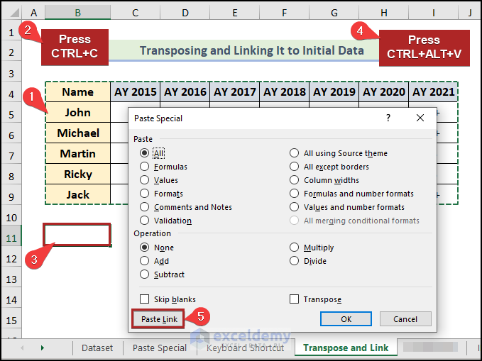
The new data set is now at the cell range of B11:I16. It’s not transposed yet. We have just linked it up with our original data set. Along with that, we see that the format is also gone. You have to redo the format unless you want it gone!
- At this moment, press CTRL + H to open the Find and Replace dialog box.
- In the Find what box, write down the equal (=) sign.
- Also, write down abc in the Replace with box.
- Lastly, click on the Replace All button.
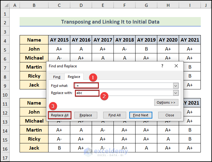
It may seem that we have lost our new data set! We’re three more steps behind our desired transposed data table.
![]()
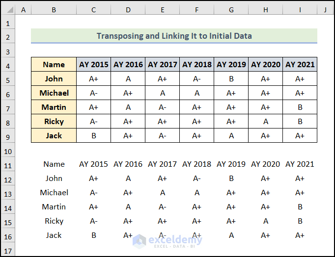
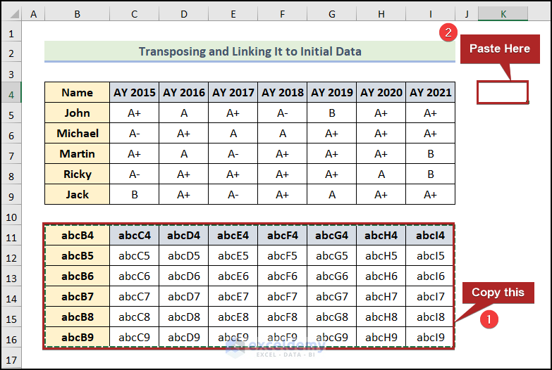
- Right now, copy the new data in the B11:I16 range.
- Then, follow the previous steps to paste them in the transposed form in cell K4.
The transposed dataset is now present in the worksheet.
![]()
- Again, bring the Find and Replace wizard like before.
- Then, write down abc and “=” in the Find what and Replace with box respectively.
- Correspondingly, click on the Replace All button.
![]()
Finally, we have generated our desired linked-up and transposed data set.
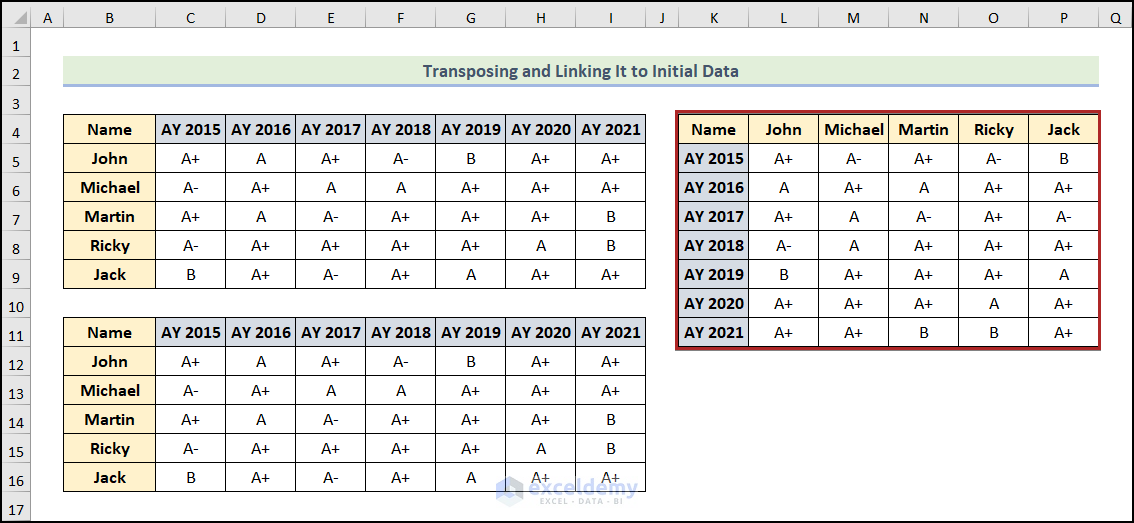
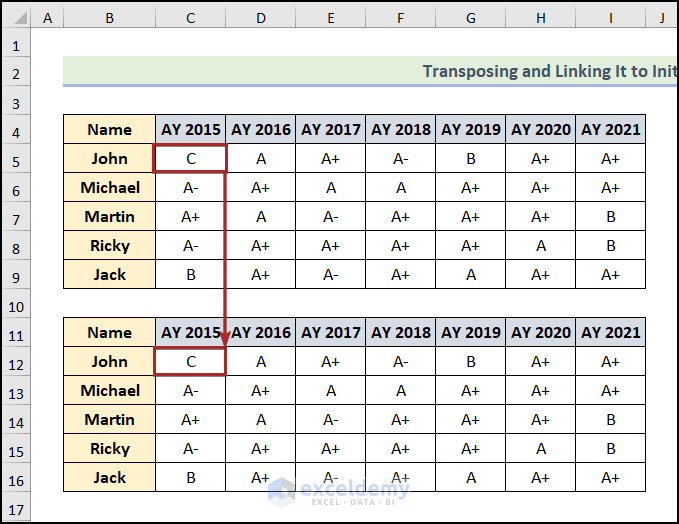
It should be noted that if you change any input in the original data set, the transposed data will also change accordingly. Look at the screenshot attached here.
Read More: How to Transpose in Excel (5 Easy Ways)
3. Applying TRANSPOSE Function
The TRANSPOSE function is very easy to use as a dynamic array in Excel 365. You can use it in other versions as well in a slightly different way. We will show that in this section. So, let’s be with us.
📌 Steps:
- Firstly, go to cell B11 and enter the following formula into the Formula Bar.
=TRANSPOSE(B4:I9)
Formula Breakdown
- Here, the COLUMN and ROW functions return the column and row number for these cell references. As example, COLUMN(B4) returns 2, ROW(B4) returns 4. So, (ADDRESS(COLUMN(B4)-COLUMN($B$4)+ROW($B$4), ROW(B4)-ROW($B$4)+COLUMN($B$4)) becomes ADDRESS(4,2).
- Output → B4
- The INDIRECT function returns the value present in the stored reference. So, INDIRECT(ADDRESS(4,2)) becomes INDIRECT(B4).
- Output → Name
- Secondly, tap the ENTER key.
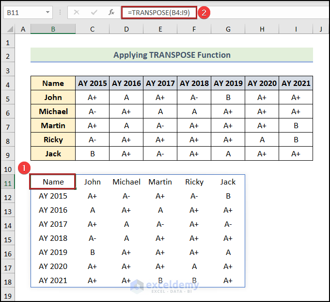
Note: The TRANSPOSE function is dynamic, which means if you change anything in the original data set, it will automatically update in the transposed output.
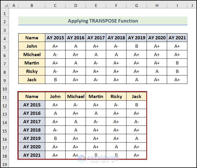
However, the formatting cannot be transferred. So, you have to do it manually.
If you don’t have MS Office 365 and have to work with the older versions of MS Excel instead, you can still work with the TRANSPOSE function. But this time it’ll be a bit less flexible for you. You have to press CTRL+SHIFT+ENTER instead of just pressing ENTER in this situation.
Read More: How to Transpose Array in Excel (3 Simple Ways)
Similar Readings
- How to Transpose Every n Rows to Columns in Excel (2 Easy Methods)
- Convert Columns to Rows in Excel Using Power Query
- How to Transpose Duplicate Rows to Columns in Excel (4 Ways)
- Transpose Multiple Columns into One Column in Excel (3 Handy Methods)
- How to Convert Multiple Columns into a Single Row in Excel (2 Ways)
4. Employing INDIRECT and ADDRESS Functions
We can also transpose rows to columns in two steps by combining the INDIRECT and ADDRESS functions. Let’s see the process in detail.
📌 Steps:
- Firstly, select cell B11 where you finally want to place the output.
- After that, type the following formula:
=INDIRECT(ADDRESS(COLUMN(B4)-COLUMN($B$4)+ROW($B$4), ROW(B4)-ROW($B$4)+COLUMN($B$4)))
- Then, press ENTER.
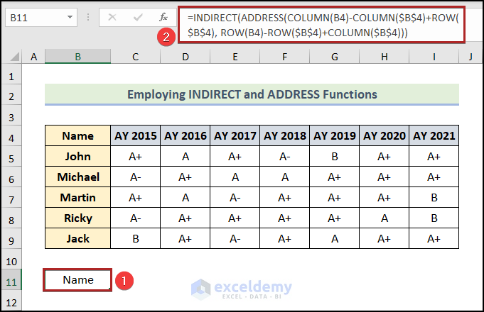
- Now, bring the cursor to the right-bottom corner of cell B11 and it’ll look like a plus (+) sign. Actually, it’s the Fill Handle tool.
- Then, drag this tool up to cell G11 in the horizontal direction.
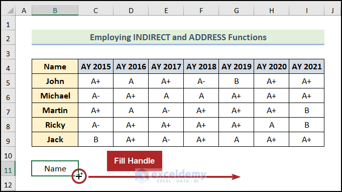
- Again, drag the Fill Handle tool up to cell G18 in the vertical direction.
![]()
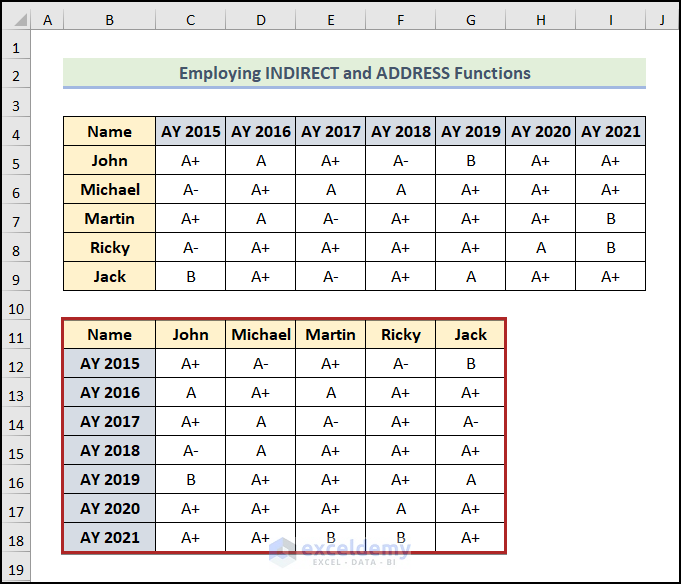
Thus, we have got the transposed data set, it’s not formatted.
![]()
The final look after formatting is like the one below.
Read More: How to Perform Conditional Transpose in Excel (2 Easy Examples)
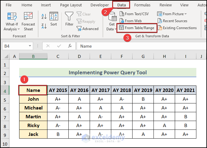
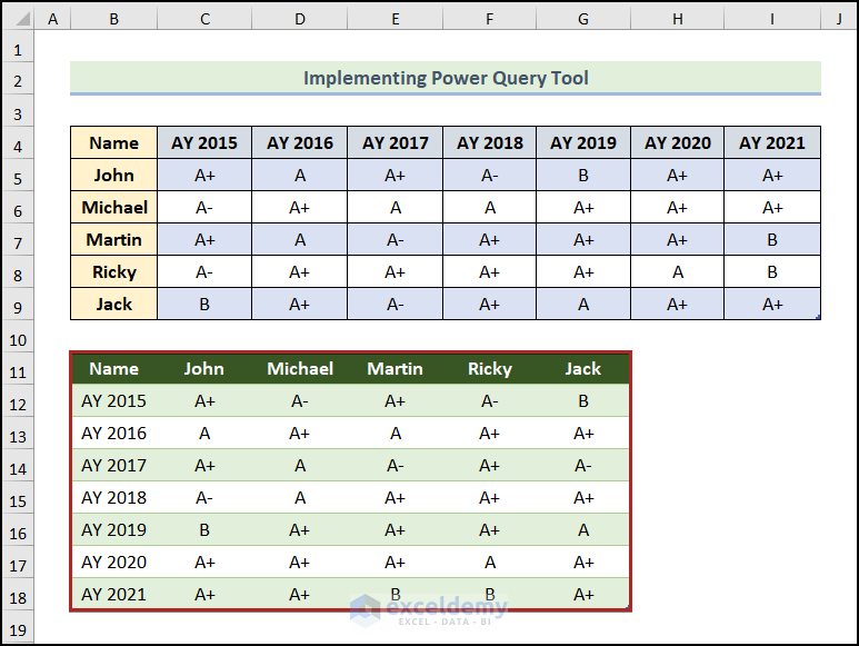
5. Implementing Power Query Tool
Power Query is a truly effective tool to transpose data quickly in Excel. This time, we will show the steps to transpose data using the Power Query tool. So, without further delay, let’s dive in!
📌 Steps:
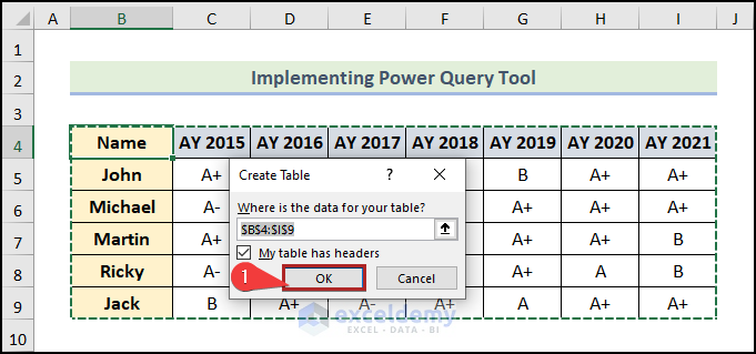
- Initially, select any cell inside the dataset. In this case, we selected cell B4.
- Then, proceed to the Data tab.
- Following this, click on From Table/Range on the Get & Transform Data group.
Instantly, the Create Table dialog box is visible before our eyes.
- Just click OK.
After a while, the Power Query Editor window will open.
- Here, advance to the Transform tab.
- Then, select Use Headers as First Row.
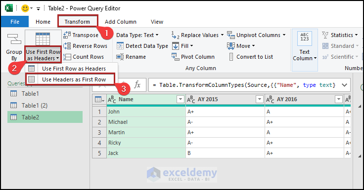
- Then, click on the Transpose feature.
![]()
- Again, jump to the Transform tab and select Use First Row as Headers.
![]()
- Henceforth, go to the Home tab.
- Then, click on the Close & Load drop-down icon.
- After that, select Cose & Load to… option.
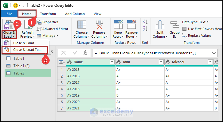
Consequently, the Import Data wizard will open up.
- Here, select the Existing worksheet as Where do you want to put the data?
- Later, give the cell reference of B11 in the box.
- Lastly, click OK.
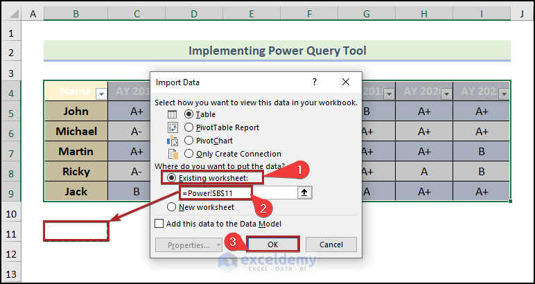
The Power Query Editor dialog box will be closed, and consequently, the transposed data will be loaded into the “Power Query“ worksheet.
Read More: Excel Power Query: Transpose Rows to Columns (Step-by-Step Guide)
6. Applying VBA Macros
Have you ever thought of automating the same boring and repetitive steps in Excel? Think no more, because VBA has you covered. In fact, you can automate the prior method entirely with the help of VBA. Let’s explore the method step by step.
📌 Steps:
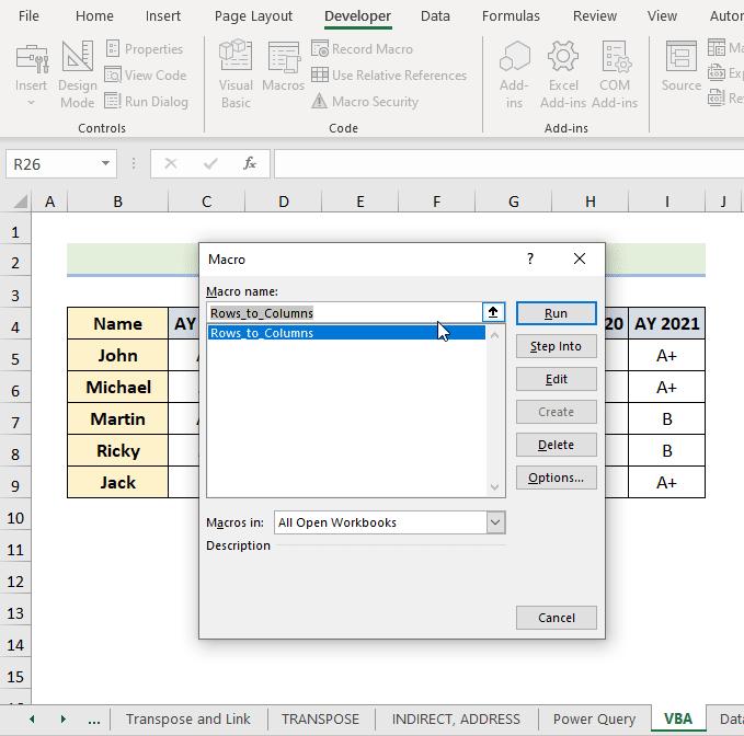
- Primarily, proceed to the Developer tab.
- Then, click on Visual Basic on the Code group.
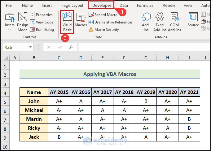
Immediately, the Microsoft Visual Basic for Applications window appears.
- Then, go to the Insert tab.
- Afterward, select Module from the options.
![]()
Instantly, Excel will insert a code module.
- Now, paste the following code into the module.
Option Explicit
Sub Rows_to_Columns()
    Dim Sr_Rng As Range
    Dim Dst_Rng As Range
    Set Sr_Rng = Application.InputBox(Prompt:="Mark the range to flip", Title:="ExcelDemy: Transpose Tool", Type:=8)
    Set Dst_Rng = Application.InputBox(Prompt:="Mark the cell where you want to place the transposed range", Title:="ExcelDemy: Transpose Tool", Type:=8)
    Sr_Rng.Copy
    Dst_Rng.Select
    Selection.PasteSpecial Paste:=xlPasteAll, Operation:=xlNone, SkipBlanks:=False, Transpose:=True
    Application.CutCopyMode = False
End Sub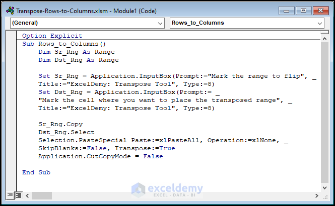
Code Breakdown
- Firstly, we mentioned the sub-procedure name. Also, declared the variables.
- Secondly, we inserted two InputBox. The values received in the InputBox will be taken by the variable.
- Thirdly, we applied the Copy method to copy the range and paste in the transposed form in the range of the second variable.
- Lastly, we ended the sub-procedure with End Sub.
- At this moment, save the file as Macro-Enabled Workbook and return to the VBA worksheet. Then, follow the GIF to understand the next procedures.
Finally, we’ve converted the rows into columns using the VBA macros.
Read More: How to Transpose Rows to Columns Using Excel VBA (4 Ideal Examples)
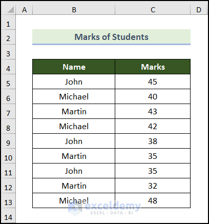
How to Transpose Rows to Columns Based on Criteria in Excel
Generally, the TRANSPOSE function may often be used to convert rows to columns. However, results depending on certain criteria, such as unique values, will not be returned. We will apply formulas combining the INDEX, MATCH, COUNTIF, IF, and IFERROR functions with arrays. So, let’s see it in action.
📌 Steps:
We are using another dataset in this example. We have the Marks of Students. This dataset contains the Name and corresponding Marks in columns B and C respectively.
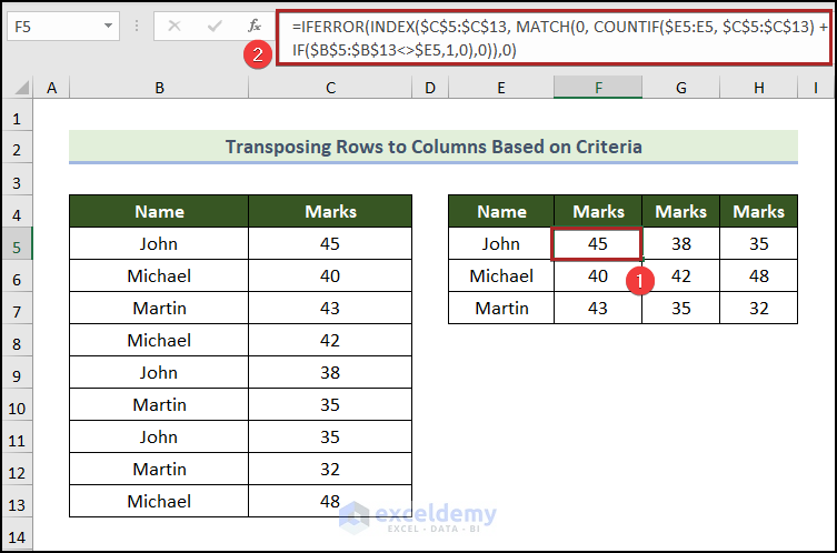
- At first, create a new table in the E4:H7 with headings Name, and Marks.
![]()
- Secondly, go to cell E5 and insert the following formula.
=INDEX($B$5:$B$13, MATCH(0, COUNTIF($E$4:$E4, $B$5:$B$13), 0))
Formula Breakdown
- COUNTIF($E$4:$E4, $B$5:$B$13) returns an array of 0 because it couldn’t find the text string Name in the B5:B13
- Then, MATCH(0, COUNTIF($E$4:$E4, $B$5:$B$13), 0) becomes MATCH(0, {0,0,0,0,0,0,0,0,0}, 0).
- Output → 1
- INDEX($B$5:$B$13, MATCH(0, COUNTIF($E$4:$E4, $B$5:$B$13), 0)) becomes INDEX($B$5:$B$13, 1).
- Output → John
- As always, press the ENTER key.
![]()
The formula used to get the marks is the following.
=IFERROR(INDEX($C$5:$C$13, MATCH(0, COUNTIF($E5:E5, $C$5:$C$13) + IF($B$5:$B$13<>$E5,1,0),0)),0)
Moreover, you can follow the article How to Transpose Rows to Columns Based on Criteria in Excel on our website to know more possible ways to do it.
Practice Section
For doing practice by yourself, we have provided a Practice section like the one below on each sheet on the right side. Please do it by yourself.
![]()
Conclusion
Now, hopefully, you’re able to transpose rows to columns in Excel in a simple and concise manner. Don’t forget to download the Practice file. Thank you for reading this article. Please let us know in the comment section if you have any queries or suggestions. Please visit our website, ExcelDemy, a one-stop Excel solution provider, to explore more.
Related Articles
- How to Transpose Columns to Rows In Excel (6 Methods)
- How to Convert Columns to Rows in Excel Based On Cell Value
- VBA to Transpose Multiple Columns into Rows in Excel (2 Methods)
- How to Swap Rows in Excel (2 Methods)
- Convert Columns to Rows in Excel (2 Methods)
- Excel Transpose Formulas Without Changing References (4 Easy Ways)

