Excel is obviously one of the most important products in the world. It is very helpful in managing, analyzing data. But there is also something that may get us frustrated when using Excel. Today I’d like to share with you some frustrating issues and how to solve them.
Although Microsoft Excel is an effective and useful software in the modern world’s activities, it has some limitations which you may face while working in it.
1. Displaying Dates in Default Format Due to Excel Limitations
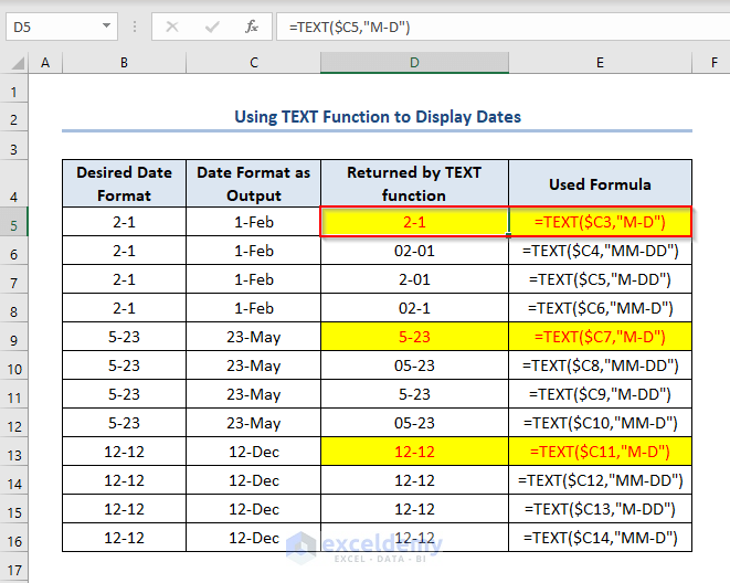
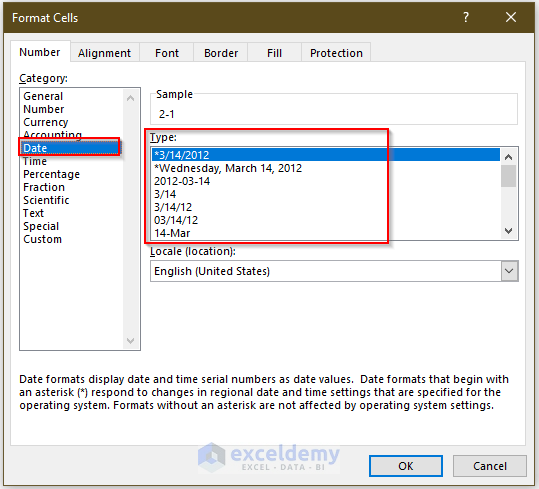
Suppose that you want to display 2-1 representing 1st Feb in Excel, what will you get after you enter 2-1 into Excel? Unfortunately, you will get 1-Feb as shown in the picture below. At this time, the method of formatting cells may come to our mind. But if we really open the Format Cells dialog box and click on Date, you will find that all formats available in the Type field are useless in our case. What should we do?
Luckily, Excel offers us the TEXT function which is much more flexible than the Format Cells dialog box. The left panel in the figure below shows you how to fix the above problem using the TEXT function. It presents three examples and what TEXT function will return with each of the four formats. If the number of digits is less than the expected number of digits, EXCEL will put leading zero before the actual number. For example, TEXT($C7,”M-D”) will return 5-23 while TEXT($C7,”MM-DD”) returns 05-23. You can look at the figure below closely and figure out what is going on behind the scenes.
And the Format Cell is like this.
In summary, the TEXT function is a good option for you to format your values. For example, you can also use the format YYYY-MM-DD to display 2015-05-23.
Read More: Advanced Excel Topics
2. Excel Limitations for Dropping Off Leading Zeros
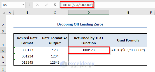
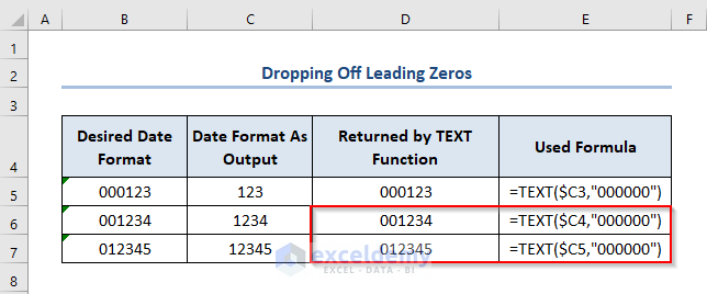
If you enter social security numbers, phone numbers, credit card numbers, or postal codes into a workbook, Excel treats them as numbers and applies a general number format to them. As a result, leading zeros are removed from those number codes. This Excel limitation occurs always. For example, you will get 123 if you enter 000123 into cell B5 of the picture below.. Similarly, Excel will display 1234 if you put 001234 into cell B6. Obviously, this is not what you want. Values in cells from B5 through B7 are what you want. Then what should you do?
Same as the above problem, we can apply the TEXT function here to pad a number code with leading zeros.
Another way to add leading zeros is to put a leading single quotation mark (‘) before number codes.
You can add the TEXT function in the D5 cell like this.
=TEXT($C5,"000000")
The output after pressing ENTER and using Fill Handle is like this.
3. Formatting Large Number as Scientific Notation
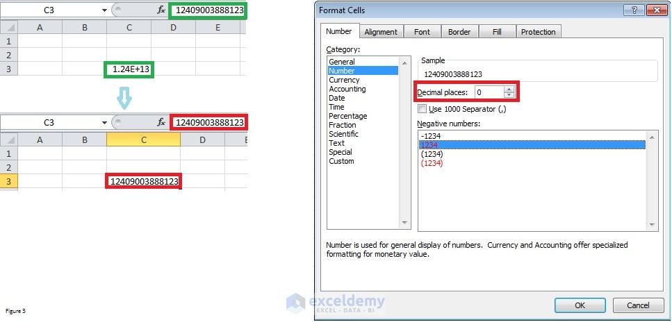
Any large number entered into Excel is stored as a number and abbreviated in scientific notation. It is a common Excel Limitation. Suppose that you put a long number like 12409003888123 in cell B2. Excel will apply a general number to it and the 12409003888123 will be presented in scientific notation as 1.2409E+13. Is it possible to prevent Excel from doing this?
The simplest way is to right-click on cell B2. Then select Format Cells to open the Format Cells dialog box. In the prompted Format Cells dialog box, select Number and set the number of decimal places as 0. So far, the long number will be displayed instead of scientific notation.
4. Using VLOOKUP Function to Approximate Match
A common Excel Limitation is many people complain that you never be sure what VLOOKUP does with an approximate match. In the picture below, if your lookup value is chun, Excel will return $93,500. When comparing against the data table in range B5:E12, you will find that this value is not what we want. In our impression, the correct value should be $151,200 as chun is similar to Chung.
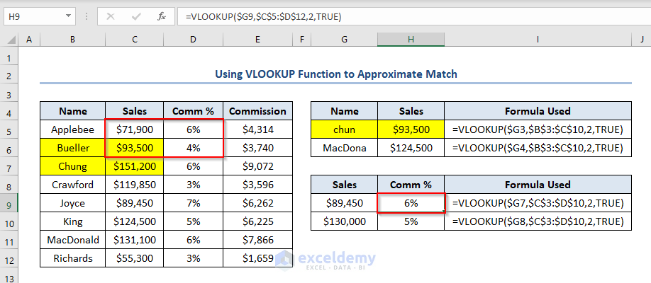
Well, VLOOKUP approximate match does not work in the way that we think. It moves through the lookup table row by row and ultimately stops on the row in which the value is less than or equal to the lookup value when the value in the next row is greater than the lookup value.
Let’s look at the above example again. Bueller is less than chun while Chung is greater than chun and therefore Excel stopped on the 6th row and returned a value $93,500 in Column C. Similarly, Excel stopped on 5th row after it reached a value $71,900 which is less than $89,450 and the value in the next row is greater than $89,450. The intersection of the 5th row and Column D gives you a commission rate of 6%.
However, if you look at the data range closely, you will find that the commission rate for $89,450 is %7. This is different from %6 that we just got from Figure 4.1. Is there anything wrong? Yes, we need to sort the lookup table ascendingly first before using the approximate match since VLOOKUP walks down the lookup table row by row.
The figure below shows another lookup table in range B5:E12. This table was sorted by Sales in ascending sequence. Now you will find that the commission rate of $89,450 is correct now.
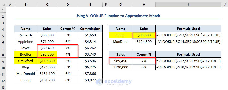
Finally, we need to remind you again. Please sort the lookup range in ascending order before using VLOOKUP approximate match. Otherwise, you will get errors.
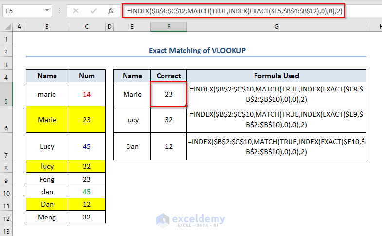
5. VLOOKUP Function Is Not Case-Sensitive
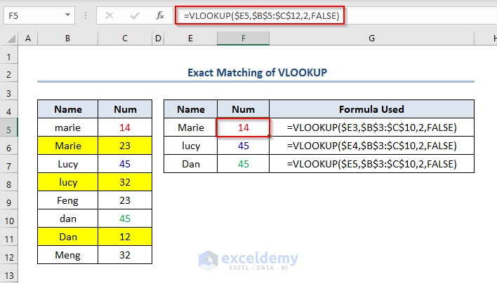
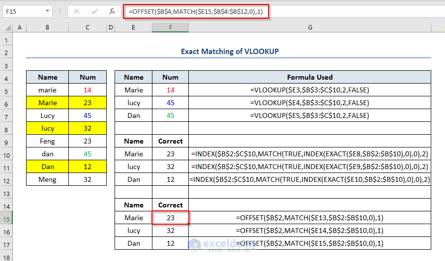
Another Excel limitation is many people are not aware that VLOOKUP is not case-sensitive and this may cause you to make mistakes. Let’s look at the figure below. marie will be matched when the VLOOKUP value is Marie and thus Excel returns 14 in cell F5. In fact, 23 in cell C6 is what we really want. How to prevent this kind of mistake from happening?
A combination of INDEX, MATCH, and EXACT functions can be used here to get the correct number 23. Range G5:G7 gives you a formula returning numbers in range F5:F7. The formula is like this.
=INDEX($B$4:$C$12,MATCH(TRUE,INDEX(EXACT($E5,$B$4:$B$12),0),0),2)
Here, MATCH(TRUE,INDEX(EXACT($E5,$B$4:$B$12),0),0) is the key to solving the problem. It gives you the row reference in which the exact match (Marie in our case) exists. Have a try on your own.
Another easier approach is to use the combination of OFFSET and MATCH functions. You can write the formula in the F15 cell like this.
=OFFSET($B$4,MATCH($E15,$B$4:$B$12,0),1)
Eventually, you’ll get an output of 23 after pressing ENTER. Simultaneously, you’ll get all the outputs by using Fill Handle.
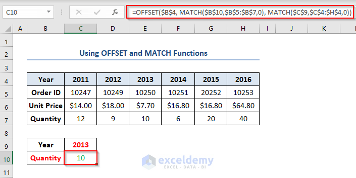
6. Cannot Start from an Arbitrary Column or Row with VLOOKUP Function
It is annoying that we can only perform a left-to-right lookup with the VLOOKUP function. But if you have read the article recommended in Section 5, you will know that the OFFSET/MATCH function can enable you to start the search from any column or row. In the following example, the value in cell C10 will change as you change the values in cells C9 and B10.
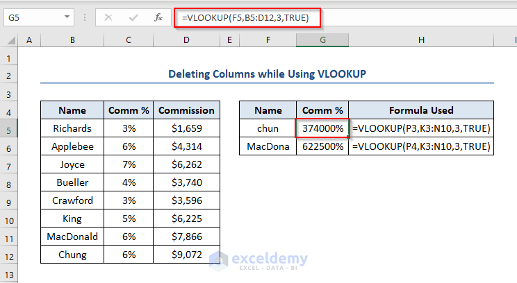
7. VLOOKUP Function Does Not Adjust Column Offset While Deleting Columns
Suppose that we have a lookup range that starts from C5 through E12. And we do VLOOKUP approximate match in range G4:I6. Let‘s take the formula in cell H5 as an example. The formula will be if we want to retrieve the approximate commission rate for chun.
=VLOOKUP(G5,B5:E12,3,TRUE)
After removing column C, you will find that the above formula will be replaced with the following formula.
=VLOOKUP(O3,K3:M10,3,TRUE)

Eventually, The lookup table was changed automatically. Even the cell reference for lookup value was also changed from “G5” to “F5”. All of these are right. But the column offset is still 3. In fact, it should be 2 as the commission rate is in the second column of the lookup table now.
8. Difficulty in View Cell’s Long Content
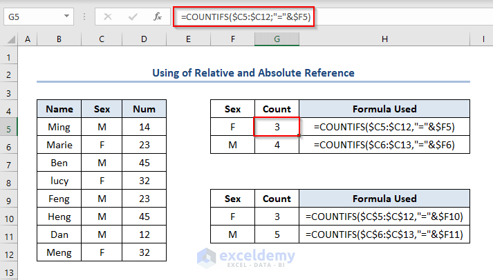
In the figure below, you will see that the cell references will change after you copy the formula =COUNTIFS($C3:$C10,”=”&$F3) from cell G3 to cell G4. The formula is =COUNTIFS($C4:$C11,”=”&$F4) in cell G4 and this formula returns 4. But if you look at range B2:D10 closely, you will find that the number of male students should be 5 instead of 4. We got a mistake here. The reason is that you apply relative reference – $C3:$C10 and it can change after you copy it to another cell. The right way here is to apply absolute reference and replace “$C3:$C10” with “$C4:$C11”. Just like what we did in range F7:H9. It’s very easy to make errors when pasting formulas and you should be careful.
9. Not Easy to View Whole Content If Cell’s Content Is Too Long
In order to illustrate this issue, I just copied a paragraph from this article into cell B6. The figure below shows you that there is only one line in the worksheet and it is difficult to view the whole content.
After adding line break inside cell B6 by pressing ALT + ENTER, we can get something like that shown in figure below. There are 11 lines now.
10. Unable to Work Seamlessly with Microsoft Word
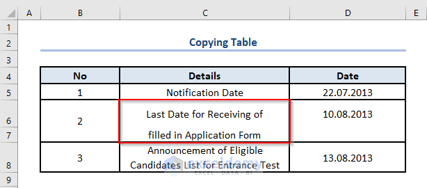
Excel splits one row containing a carriage return into multiple rows when copying a table from Word into Excel. Suppose that there is a doc file – Copy table from word to excel.docx – containing the below table.
| No | Details | Date |
|---|---|---|
| 1 | Notification Date | 22.07.2013 |
| 2 | Last Date for Receiving of
filled in Application Form |
10.08.2013 |
| 3 | Announcement of Eligible Candidates List for Entrance Test | 13.08.2013 |
If we copy this table into a worksheet using CTRL+C and CTRL+V, we will get something like that shown in Figure 10.1. You can see that the Last Date for Receiving of filled in Application Form is split into two rows. This is absolutely not what we want.
To prevent this from happening, we can use VBA macro to extract tables from Word files into Excel files. The code in the following table can retrieve data from all the tables within a word document into an Excel file.
Sub Import_Table()
Dim wdDoc As Object
Dim wdFileName As Variant
Dim tableNo As Integer   'table number in Word
Dim iRow As Long    'row index in Excel
Dim iCol As Integer    'column index in Excel
Dim resultRow As Long
Dim tableStart As Integer
Dim tableTot As Integer
On Error Resume Next
ActiveSheet.Range("A:AZ").ClearContents
wdFileName = Application.GetOpenFilename("Word files (*.docx),*.docx", , _
"Browse for file containing table to be imported")
If wdFileName = False Then Exit Sub '(user canceled import file browser)
Set wdDoc = GetObject(wdFileName) 'open Word file
With wdDoc
tableNo = wdDoc.tables.Count
tableTot = wdDoc.tables.Count
If tableNo = 0 Then
MsgBox "This document contains no tables", _
vbExclamation, "Import Word Table"
ElseIf tableNo > 1 Then
tableNo = InputBox("This Word document contains " & tableNo & " tables." & vbCrLf & _
"Enter the table to start from", "Import Word Table", "1")
End If
resultRow = 1
For tableStart = 1 To tableTot
With .tables(tableStart)
'copy cell contents from Word table cells to Excel cells
For iRow = 1 To .Rows.Count
For iCol = 1 To .Columns.Count
ThisWorkbook.Worksheets("Import_Table").Cells(resultRow, iCol) = WorksheetFunction.Clean(.cell(iRow, iCol).Range.Text)
Next iCol
resultRow = resultRow + 1
Next iRow
End With
resultRow = resultRow + 1
Next tableStart
End With
End Sub
After clicking on the Import table button, we will get a table similar to that in Figure 10.2. I changed the column width here manually to demonstrate that “Last Date for Receiving of filled in Application Form” was not split into two rows.

11. Taking a Long Time Sometimes While Recalculation of Formulas
Excel recalculates your workbook’s formulas when you open the workbook or when you make significant changes. This feature is good but these recalculations can take a long time. It is not so good from this point of view. Below are two approaches for you to control calculation and save your time.
♦ Turn Off Automatic Recalculation
Firstly, click on the File tab -> Options.
Secondly, click the Formulas category.
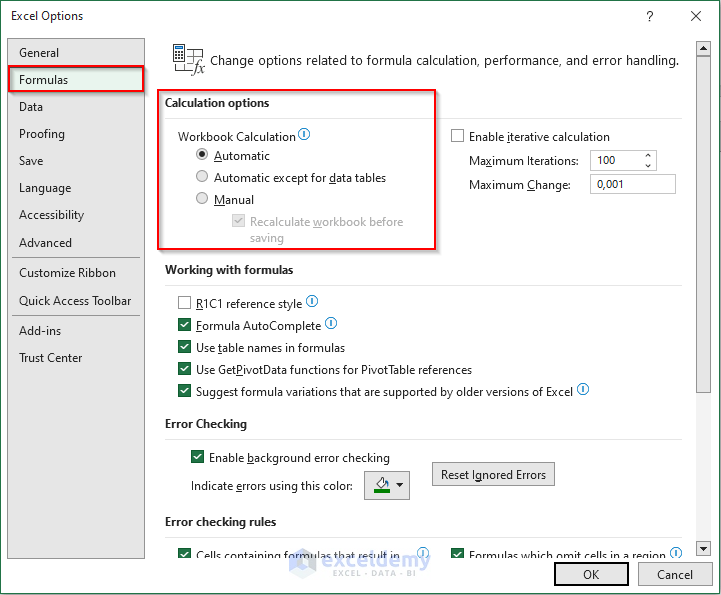
You will get an Excel Options dialog box as shown in the figure below. Automatic under Workbook Calculation in the Calculation options section means that Excel will recalculate all dependent formulas every time you make a change to a value, formula, or name. Automatic except for data tables means that Excel will recalculate all dependent formulas except for data tables. The last choice Manual can enable you to turn off automatic recalculation.
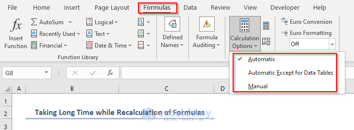
The figure below presents another method to turn off automatic recalculation. There are also three options for you to choose.
- Automatic,
- Automatic Except for Data Tables, and
- Manual.
Eventually, after you turn off automatic recalculation, you can click the Calculate Now button in the Calculation group on the Formulas tab. This method. can enable Excel to recalculate all open worksheets. Another option – Calculate Sheet button – can make Excel recalculate active worksheets and any charts/chart sheets linked to this worksheet.
♦ Change the Number of Times Excel Iterates a Formula
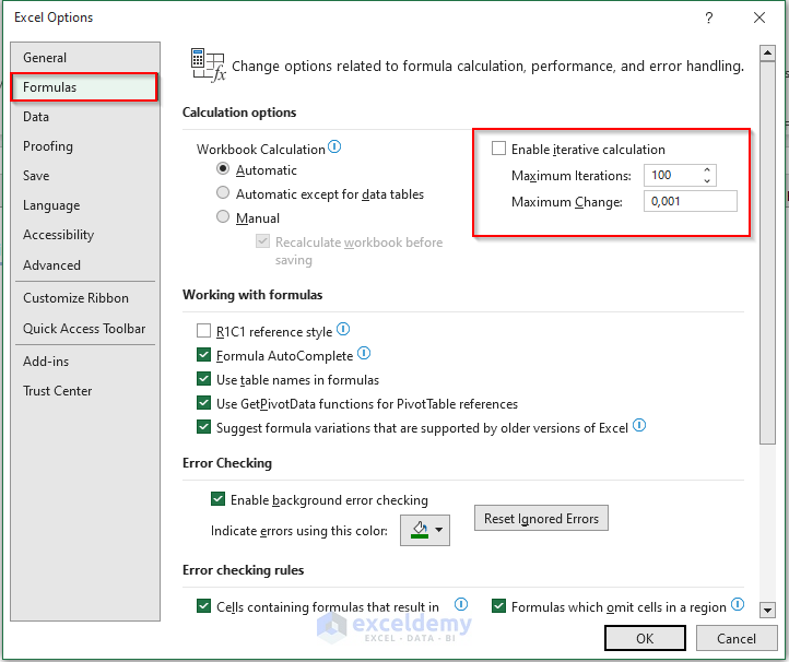
Please make sure Enable iterative calculation check box was selected before you set maximum iterations and maximum change. The higher the number of iterations, the more time Excel will need to recalculate a worksheet. The smaller the maximum amount of change, the more accurate the result and the more time Excel needs to recalculate a worksheet.
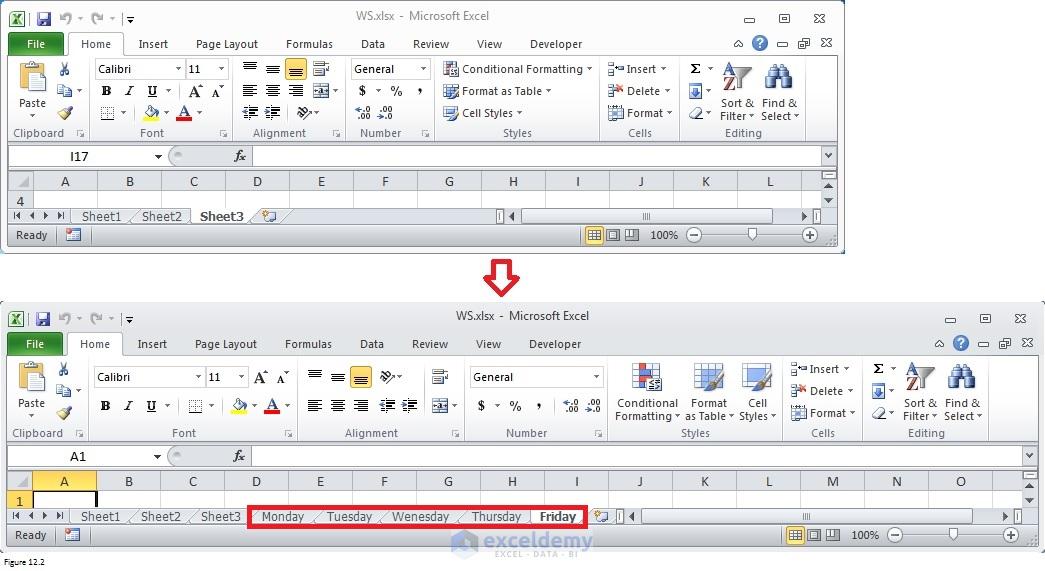
12. Limited Ways to Rename Multiple Excel Worksheets
Sometimes, we need to insert multiple worksheets. What will you do to rename all of those worksheets? Use Rename command to rename them one by one? What if you have to rename 100 worksheets? It will take you a lot of time to finish the task. Luckily, we can use the VBA code for renaming multiple worksheets.
Here is the code for inserting and renaming multiple worksheets.
Sub rename_tab()
Application.DisplayAlerts = False
'Define variable
Dim wbk As Workbook
Dim ws As Worksheet
'Open workbookFile
Set fnm = ThisWorkbook.Sheets(1).Cells(1, 2)
Set wbk = Workbooks.Open(fnm)
'Set workbook as active workbook
wbk.Activate
For i = 2 To ThisWorkbook.Worksheets(2).UsedRange.Rows.Count
'Return number of all worksheet in the active workbook
n = Worksheets.Count
'Add worksheet after the last worksheet
Set ws = Sheets.Add(After:=Worksheets(Worksheets.Count))
'Give the newly added worksheet a name
ws.Name = ThisWorkbook.Worksheets(2).Cells(i, 2)
Next i
'Close and save active workbook
wbk.Close Savechanges:=True
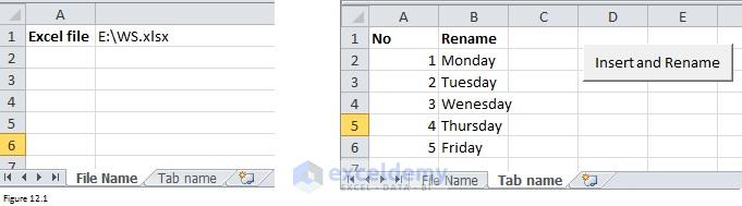
End SubThe figure shows you how to design and use this macro. Suppose that the macro was saved in Insert and Rename Multiple Tabs.xlsm files. There are two tabs in this xlsm file. The first one is to include a file in which you want to insert tabs. You need to enter the file pathname into cell B1. The macro will open the file listed in cell B1 (WS.xlsx in our case). The second worksheet (right panel of the figure) provides tab names that will be used by VBA macro. You can add as many tab names to the second worksheet.
The figure below presents the screenshots for WS.xlsx before and after running the above VBA code.
13. Limitations in Excel PivotTables That Do Not Have Median
A PivotTable is one of the most powerful features. It allows you to summarize, analyze, explore and present your data. It helps you extract significant insight and detailed data sets.
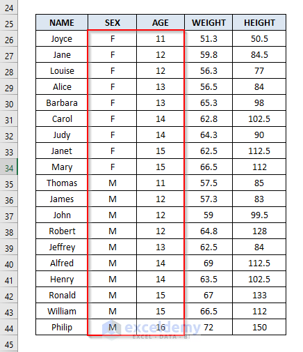
The left panel in the figure below contains data to be analyzed in our case. You can see that we have height and weight for different students as well as their sex and age.
Firstly, click any cell in the range B5:F23.
Secondly, on the Insert tab, click PivotTable.
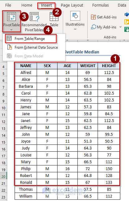
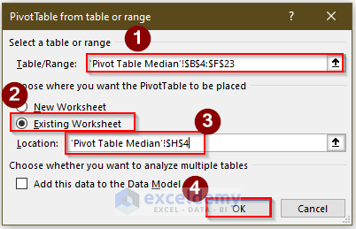
Thirdly, choose the default location in the prompted Create PivotTable dialog box. You can see that this range is selected in the middle panel of the figure.
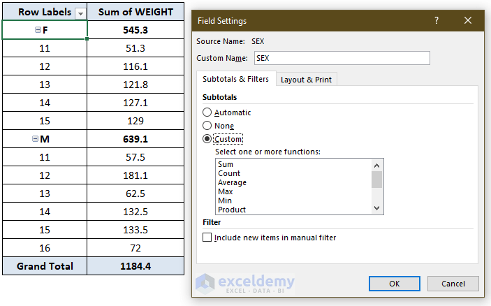
In the appeared PivotTable field list dialog box (right panel of the figure below ), drag SEX and AGE to the Row Labels area. Then drag WEIGHT to the Values area. Finally, a PivotTable including cells from H5 through I19 was created.
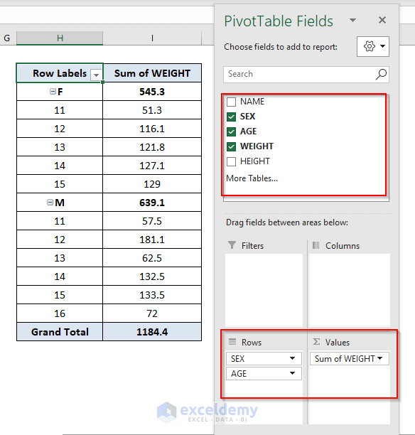
Eventually, from the pivot table, the sum of weight for male students who are 11 is 57.5. And the sum of weight for female students who are 13 is 121.8.
Additionally, the sum statistics, we can also count the number of students who are 13 or compute the average weight. Right-click on any cell in the pivot table (range H5:I19) and then choose Value Field Settings. In the Value Field Settings dialog box (right panel of the figure ), you can select the type of calculation in which you are interested.
Importantly, the type of calculation includes Count, Average, Max, Min, etc. If you read through all types of calculations, you will notice that EXCEL does not provide the Median statistics in the PivotTable. Then what should we do if we really want to calculate Median statistics? A MEDIAN function is a good option.
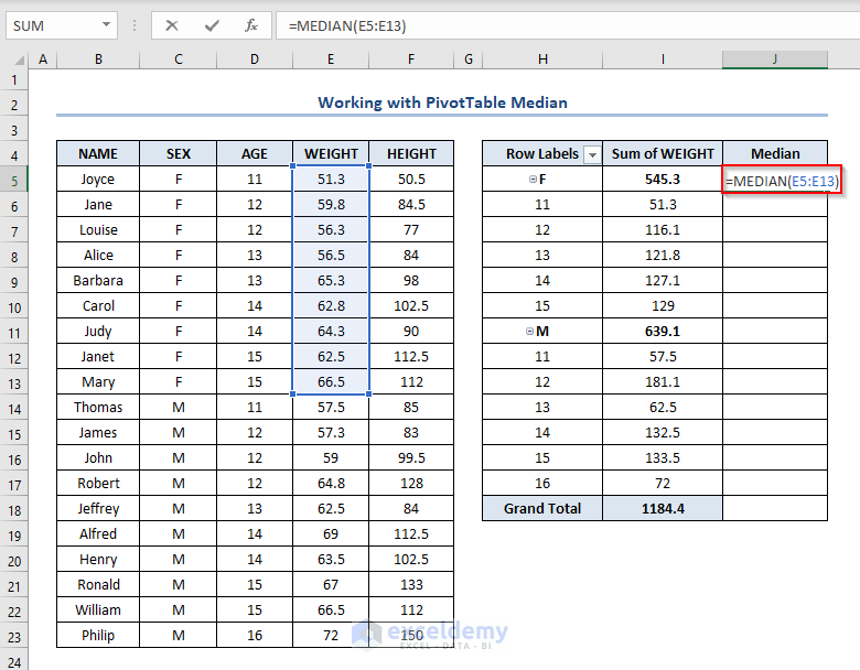
Before using the MEDIAN function, it is better to sort data by SEX and AGE. Here, we have sorted the dataset according to SEX and AGE.
Now let’s use the MEDIAN function to calculate the Median for each subgroup. The formula in cell J5 is like this.
=MEDIAN(E27:E35)
Here, E27:E35 refers to the WEIGHT of the female students.
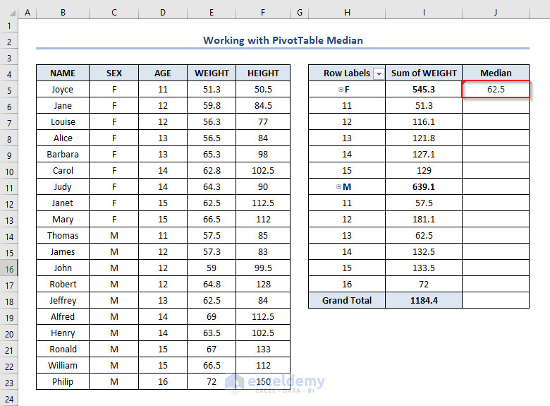
Eventually, after pressing ENTER it returns 62.5. It tells that the Median WEIGHT for female students whose age is between 11 and 15 is 62.5 kg.
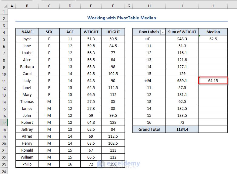
Similarly, you need to write the formula below in the case of male students.
=MEDIAN(E14:E23)
Here, E14:E23 refers to the WEIGHT of male students.
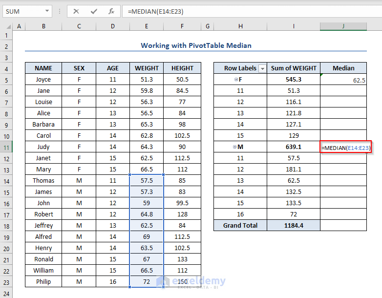
Repeatedly, if you press ENTER you’ll find the output as 64.15.
14. Excel PivotTables Limitations for Not Counting Unique Values
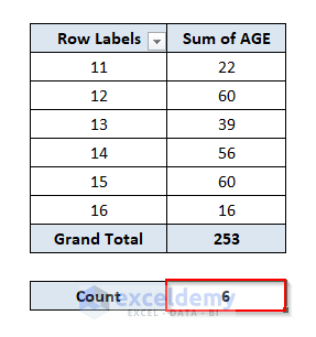
Sometimes, we may want to find out how many unique values exist in a range that contains duplicate values. But PivotTables do not count unique values. The figure below illustrates this. You can find that there are 2 students who are 11 years old and 5 students who are 12 years old. But if you want to know the range of age distribution, you have to count one by one manually.
Firstly, you have to make a PivotTable. Suppose the PivotTable is with Row Levels and Sum of AGE.
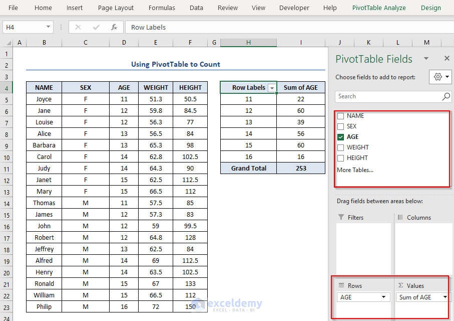
Secondly, you can use the ROWS function which can return the number of rows in the reference range. You need to write the formula like this.
=ROWS(H5:H10)
Here, H5:H10 refers to the Row Levels.
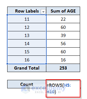
Eventually, press ENTER to get the output as 6.
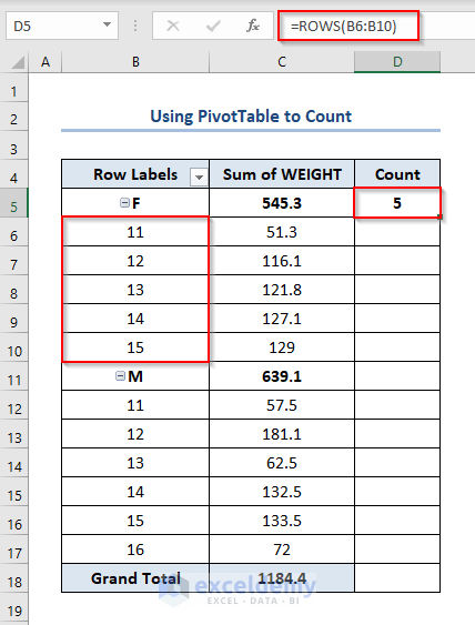
And here Figure below shows you how to count unique values for different sex groups. What we did here is to apply the ROWS function to each subgroup. For the female group, enter the formula like this into cell D5.
=ROWS(B6:B10)
Similarly, press ENTER to get the count as 5.
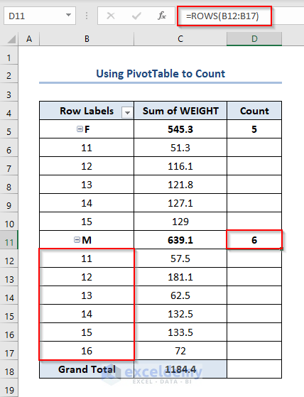
And for the male group, enter the formula into the D11 cell like this.
=ROWS(B12:B17)
Eventually, it will return 6.
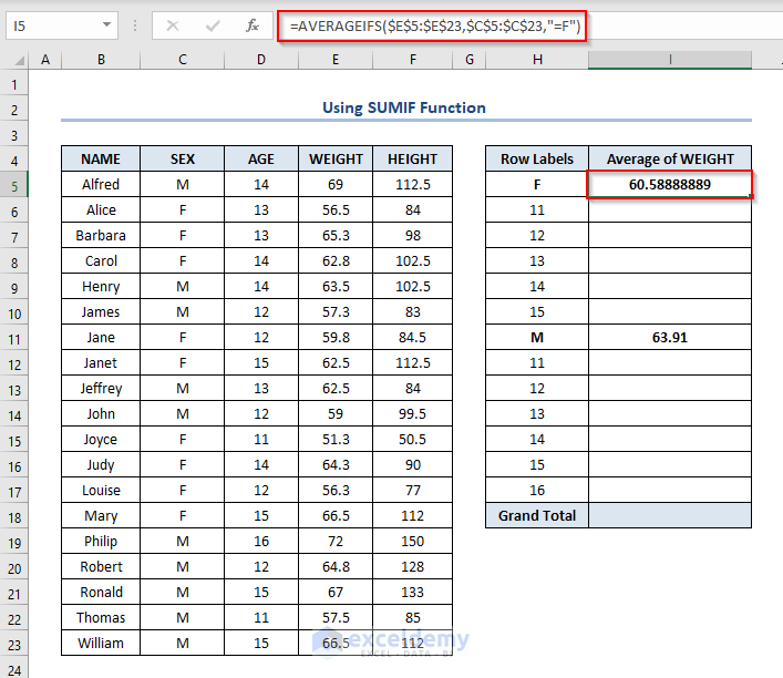
15. No SUMIF / COUNTIF / AVERAGEIF Equivalents for Functions Such as Max Or Median
The SUMIFS function can sum cells meeting multiple criteria. The SUMIF function can only apply one criterion while the SUMIFS function can be applied to more than one set of criteria with more than one range.
The Sum_range argument in the function means the range to be summed. Criteria_range and criteria are provided in pairs.
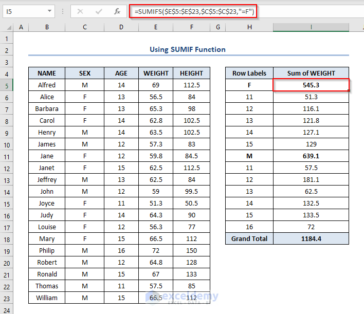
Mainly, the formula for the I5 cell is.
=SUMIFS($E$5:$E$23,$C$5:$C$23,"F=")
The sum range for cell I5 is E5:E23. The first criterion is C5:C23,”= F” while the second criterion is E5:D23,= 11. The sum of weights for female students who are 11 years old is 51.3 kg.
Generally, the AVERAGEIFS function has a similar syntax to SUMIFS. The figure below shows you how to use the AVERAGEIFS function.
Additionally, the COUNTIFS function is slightly different from the SUMIFS function and AVERAGEIFs function.
Importantly, the syntax only consists of different pairs of criteria_range and criteria. The range like sum_range or average_range should be removed. The figure below shows you how to apply the COUNTIFS function.
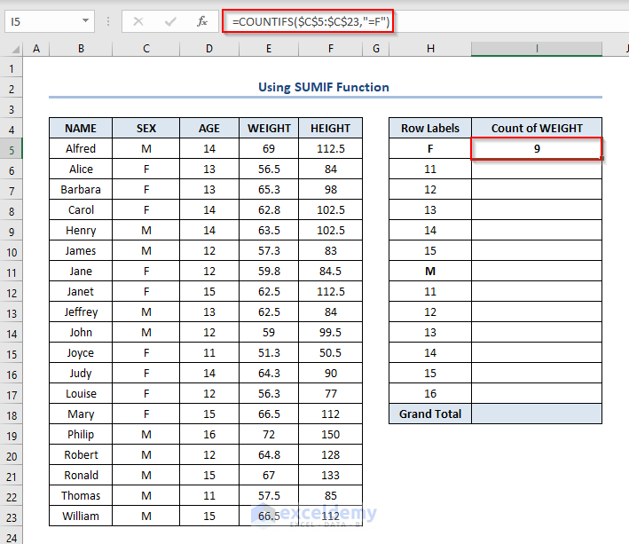
Eventually, these functions are useful, right? However, there is no equivalent function like the MEDIANIFS function.
16. Features Available in Excel for Windows When Limited for Mac
Some useful reporting features do not work in Excel for Mac and thus you cannot use them when generating reports for clients who use Mac. Besides these reporting features, there are also other features that are incorporated into the Windows version of Excel but are not included in the Mac version of Excel.
For example, Excel for Windows allows you to set a default location for saving files. It can automatically save draft copies of your workbook as you work to minimize your loss if Excel crashes suddenly. Windows version of Excel can also allow you to customize the Quick Access Toolbar. All these three features are not supported by Excel for Mac.
Generally, with Excel for Windows, you can preview the workbook in three modes.
- Normal
- Page Layout and
- Page Break.
Eventually, with Excel for Mac, you can only use Normal and Page Layout preview mode. As for the Print Preview, you can see a large print preview of the workbook and zoom in or out in the windows version of Excel. But for Excel on Mac, you can only see a small Print Preview which cannot be zoomed. The View Side by Side feature which allows you to compare two workbooks easily is only available in the Windows version of Excel. And the Synchronous Scrolling that allows you to scroll through two workbooks at the same time is also missing in Excel for Mac.
17. Cannot Quick Access to Tables in Excel Options Dialog Box
If you open the Excel Options dialog box, you will find that there are 10 tabs and each of them is filled with dozens of settings. Locating a specific can waste considerable time.
18. Specification Limits of Excel
It is well known that Excel has limits. For example, whether the workbook can be opened will be limited by available memory and system resources. The maximum number of rows is 1,048,576 and the maximum number of columns is 16, 384.
But some limitations are annoying. For instance, the maximum number precision is 15. It means that the number of digits a cell can contain is only 15. Excel will replace digits (after the 15th digit) with zeros. If you enter 12345678901234567890 into a cell, you will get 12345678901234500000 instead.
19. Limitations in Spell Checking in Excel
Microsoft Word offers automatic spell checking which can check the spelling and grammar of your files. It can highlight the mistakes. However, Excel does not automatically highlight the mistake. But using the Reviews > Proofing > Spelling command, you can check out the errors with your Excel files.
20. Excel Crushes Easily When Running Macros
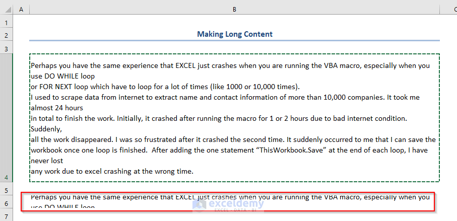
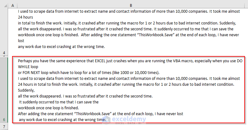
Perhaps you have the same experience that Excel just crashes when you are running the VBA macro, especially when you use the DO WHILE loop or FOR NEXT loop which has to loop a lot of times (like 1000 or 10,000 times). I used to scrape data from the internet to extract the names and contact information of more than 10,000 companies. It took me almost 24 hours in total to finish the work. Initially, it crashed after running the macro for 1 or 2 hours due to bad internet conditions. Suddenly, all the work disappeared. I was so frustrated after it crashed the second time. It suddenly occurred to me that I can save the workbook once one loop is finished. After adding the one statement “ThisWorkbook.Save” at the end of each loop, I have never lost any work due to excel crashing at the wrong time.
21. CSV File Related Excel Issue
Excel has CSV file format issues. Sometimes, users using Excel 2013 and 2016 with language variation try to open a CSV file generated from a US application by double clicking on it. But Excel doesn’t format the file and shows it in CSV mode (comma separate) by default. Excel employs the List Separator character (such as a comma, semicolon, etc.) for regions. The solution to this may be.
- Select a region that uses a comma as a list separator (i.e. USA, Canada, etc.)
- Open and Create the CSV file in Excel and save it as a worksheet.
- Return the regional settings back to the original state.
22. Excel Limitations for Data Analytics
While data analysis in Excel you will face difficulties because of the issues.
- Excel limits visibility when creating complex models.
- Excel limitations make collaboration more challenging
- Excel is inefficient in managing templates and data entry
- Limitations of Excel make keeping track of multiple spreadsheets challenging.
Read More: Basic Terminologies of Microsoft Excel
Download Practice Workbook
Conclusion
The purpose of this article is to focus on some important limitations of working with Excel. There may be some other limitations too.
Get FREE Advanced Excel Exercises with Solutions!

19 Excel does have Spell Check… (under Review) 😉
Yes. Corrected.
Thanks, Luke for the tips.