SUMPRODUCT is one of the most powerful array functions in Microsoft Excel that can pull out data from an array based on the criteria along multiple columns & rows. In this article, you’ll learn how to use this SUMPRODUCT function with multiple columns under a number of criteria in an efficient manner.
Introduction to SUMPRODUCT Function
Before getting down to the uses of the SUMPRODUCT function, let’s have a look at first how this function works.
- Syntax:
- Output:
- Example:
In our example below, there are two columns comprising of unit & cost per unit of some materials. With the SUMPRODUCT function, we can easily find out the total cost for all units. To do this, we have to type in cell C7:
=SUMPRODUCT(B3:B6*C3:C6)After pressing ENTER, you’ll get the total cost at once for all products.
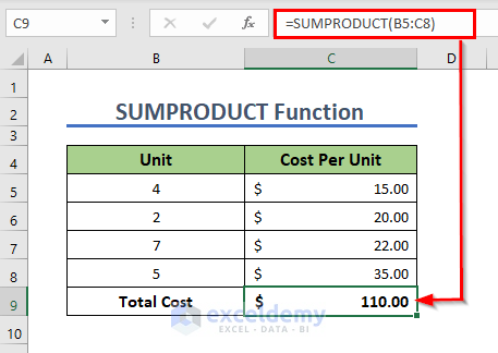
Inside the SUMPRODUCT function, we’re technically multiplying all units from Column B with the related costs per unit from Column C. The SUMPROUCT function will then return by summing up all the products.
How to use SUMPRODUCT Function with Multiple Columns in Excel: 4 Suitable Approaches
We will now try to demonstrate 4 different approaches to applying the SUMPRODUCT function in Excel under different criteria. Let’s start!
1. Using SUMPRODUCT with Multiple Columns Under AND Logic Criteria
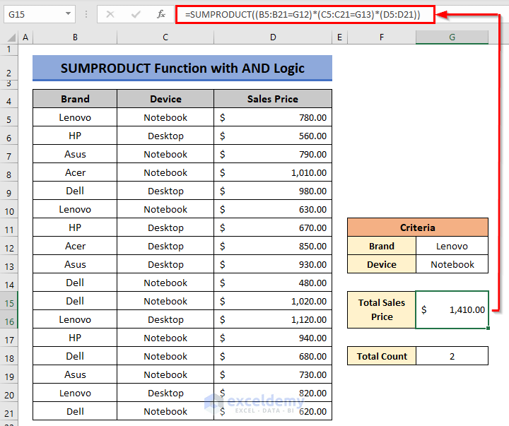
Now we’ll deal with our actual dataset where 3 columns are present with computer brands, device categories & sales price for each. In our first application with the SUMPRODUCT function, we’ll find out the total sales price of the Lenovo notebook from the table data.
📌 Steps:
- First of all, select cell G15, and type the following formula:
=SUMPRODUCT((B5:B21=G12)*(C5:C21=G13)*(D5:D21))
- Now, press ENTER, and you’ll get the result at once.
💡 How the Formula Works
B5:B21=G12 matches cell G12 (i.e. Lenovo) with the range B5:B21 & C5:C27=G13 also matches cell G13 with the range C5:C27 and returns TRUE or FALSE. Matching both ranges, the total price of Notebook device of the Lenovo brand is calculated inside the function.
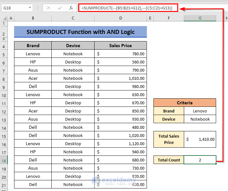
With the SUMPRODUCT function, we can also extract the total counts of Lenovo notebooks or any other category from the table.
📌 Steps:
- First, select cell G18, and type:
=SUMPRODUCT(--(B5:B27=G12),--(C5:C27=G13))
- Then, press ENTER, and you’ll see the result right away.
💡 Formula Explanation
In this case, we’re using logic arguments inside the SUMPRODUCT function. We’re asking the function to determine if the selected criteria match the cell values in Columns B & C. Uses of Double-Unary(–) before the arguments will convert the logical text values (TRUE or FALSE) into 1 or 0. And then SUMPRODUCT will sum up those number values to display the final result.
Read More: How to Use SUMPRODUCT with Criteria in Excel
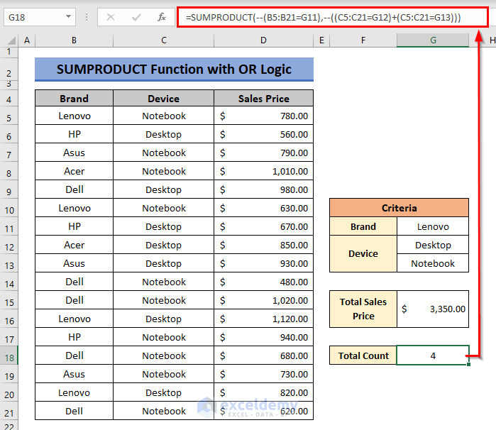
2. Using SUMPRODUCT with Multiple Columns Under OR Logic Criteria
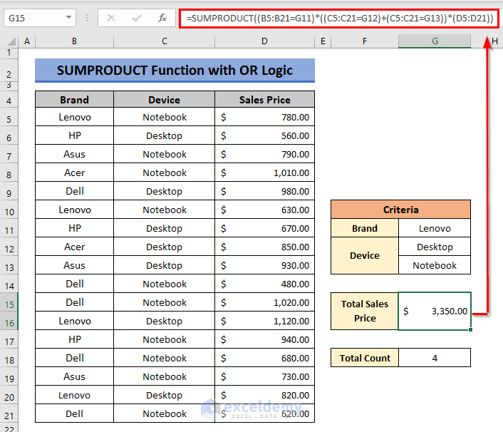
Now we’ll assign OR logic in our criteria. We’ll determine the total sales price of the Lenovo notebook and desktop.
📌 Steps:
- First, type the formula below in cell G15.
=SUMPRODUCT((B5:B21=G11)*((C5:C21=G12)+(C5:C21=G13))*(D5:D21))
- Now, press ENTER, and the total sales price will be displayed in that cell.
💡 How the Formula Works
B5:B21=G11 matches cell G11 (i.e. Lenovo) with the range B5:B21 & C5:C27=G12 matches cell G12 with the range C5:C27 & D5:D27=G13 matches cell G13 with the range D5:D27 and returns TRUE or FALSE. Matching both ranges, the total price of the Notebook and Desktop of the Lenovo brand is calculated inside the function.
If we want to count the presence of Lenovo devices in the table, then the device criteria will have to be added by inserting a Plus(+) between those two criteria.
Just apply the formula below in cell G18.
=SUMPRODUCT(--(B5:B27=G11),--((C5:C27=G12)+(C5:C27=G13)))
Read More: How to Use SUMPRODUCT IF in Excel
3. Using SUMPRODUCT Along Multiple Columns and Rows
SUMPRODUCT is one of the most useful functions that can extract data or do complex calculations by scrutinizing all mentioned criteria along rows & columns from an array. In our following & new dataset, the sales of computer devices of different brands are presently based on the months. We’ll find out the number of sales for HP notebooks in January.
The SUMPRODUCT function can extract data or do complex calculations by scrutinizing all mentioned criteria along rows & columns from an array. In our following & new dataset, the sales of computer devices of different brands are presently based on the months. We’ll find out the number of sales for HP notebooks in January.
All you have to do is apply the following formula in cell L11 and you’ll get the total counts instantly under our criteria.
=SUMPRODUCT(D5:I14,(C5:C14=C10)*(D4:I4=L9)*(B5:B14=L7))
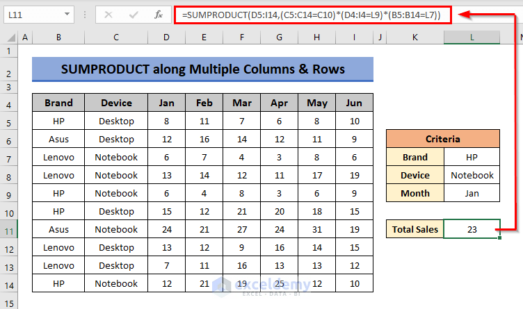
💡 Formula Explanation
If you look carefully inside the function, we’ve selected the entire array of sales data first. Then we added the criteria along 2 columns and a row. SUMPRODUCT function then looked for our criteria in the selected array and returned the final result by summing up all extracted data.
Read More: How to Use SUMPRODUCT to Lookup Multiple Criteria in Excel
4. Inserting SUM Function Inside SUMPRODUCT to Calculate Weighted Average
By combining the SUMPRODUCT, and SUM functions together, we can determine the weighted values for a range of data. The following dataset represents a student’s final exam marks along with the assigned weights of a number of subjects. We’ll calculate the weighted average marks of the student.
The formula to find the weighted average in cell F8 will be:
=SUMPRODUCT(C5:C11*D5:D11)/SUM(D5:D11)
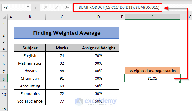
So, here the SUMPRODUCT function sums up all the products of marks & assigned weights. Then the calculated result will be divided by the summation of all assigned weight percentages.
Related Content: Excel SUMPRODUCT Function Based on Date Range
Download Practice Workbook
You can download our Excel workbook that we’ve used to prepare this article.
Concluding Words
I hope this article on the uses of the SUMPRODUCT function along multiple columns will now prompt you to apply it in your regular Excel chores. If you got any questions or suggestions let me know through comments. You can check out our other interesting articles related to Excel functions on this website.
Related Articles
- SUMPRODUCT Across Multiple Sheets in Excel
- SUMPRODUCT for Counting with Multiple Criteria in Excel
- [Solved] SUMPRODUCT with Multiple Criteria Not Working in Excel
- Excel SUMPRODUCT with Multiple Criteria in Same Column
<< Go Back to Excel SUMPRODUCT Function | Excel Functions | Learn Excel
Get FREE Advanced Excel Exercises with Solutions!

Hi, thank you for your help. Thought you might like to know that your formula
=SUMPRODUCT(D5:I14,(C5:C14=C10)*(D4:I4=L9)*(B5:B14=L7))
should be;
=SUMPRODUCT(D5:I14,(C5:C14=L8)*(D4:I4=L9)*(B5:B14=L7))
Hello, MARK EVANS!
You have pointed out a fantastic thing.
Your reference is correct. We had an unfortunate mistake in the reference to this formula. There will be L8 at the reference in the place of the C10 reference.
Thank you for your valuable feedback. We appreciate it so much.
So, the formula should be:
=SUMPRODUCT(D5:I14,(C5:C14=L8)*(D4:I4=L9)*(B5:B14=L7))Regards,
Tanjim Reza
This was LIFE CHANGING. I thought I was good at Excel til I saw this. My god!
Hi,
regarding:
1. Using SUMPRODUCT with Multiple Columns Under AND Logic Criteria
what if I want to see not 1 brand, but 2 or 3 brands?
Thank you in advance!
Hello ALEQ,
Thank you for your query. If you want to sum one specific product of two or three brands you just have to use an OR logic for brands.
Let us assume we want to find the sum of notebook sales of Lenovo and Asus brands. For that insert the following formula:
=SUMPRODUCT(((B5:B21=G12)+(B5:B21=G13))*(C5:C21=G14)*(D5:D21))
Here, (B5:B21=G12)+(B5:B21=G13), this part applies the OR logic for brands. It matches the range B5:B21 with G12 and G13 cell values and returns TRUE or FALSE. So, it returns TRUE for Lenovo and Asus brands and Excel counts them as 1.
Similarly, C5:C21=G14 returns TRUE or 1 for if any match is found and D5:D21 simply returns the sales values.
So, the function sums up the prices of notebooks of two different brands.
If you want to sum up prices for more brands, then just add another logic that matches brands in this part “(B5:B21=G12)+(B5:B21=G13)” of the formula.
Regards,
Priti
Exceldemy Team
How would I add months together like JAN & FEB in the formula but keeping the data range the same.
Hi TRICIA,
Thank you for your comment. To add the sales of JAN & FEB you can use this formula:
=SUMPRODUCT(D5:I14,(C5:C14=C10)*(D4:I4=L9)*(B5:B14=L7))+SUMPRODUCT(D5:I14,(C5:C14=C10)*(D4:I4=L10)*(B5:B14=L7))Regards,
Mahfuza Anika Era
Exceldemy Team