Excel is part and parcel of our daily life. When we think about data, the first thing that comes to our mind is Excel. We can do all sorts of data manipulation with Excel. When working with large amounts of data, we need to use the SUMIFS function. In this article, we will discuss the use of SUMIFS with multiple criteria along the column and the row in Excel.
Introduction to SUMIFS Function in Excel
The SUMIFS function is a math and trig function. It adds all of its arguments that meet multiple criteria.
- Function Objective:
Add the cells given by specified conditions or criteria.
- Syntax:
=SUMIFS(sum_range, criteria_range1, criteria1, [criteria_range2, criteria2], ...)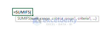
- Arguments Explanation:
| Arguments | Required/Optional | Explanation |
|---|---|---|
| sum_range | Required | Range of cells that has to be summed under conditions or criteria. |
| criteria_range1 | Required | Range of cells where the criteria or condition will be applied. |
| criteria1 | Required | Condition for the criteria_range1. |
| [criteria_range2] | Optional | 2nd range of cells where the criteria or condition will be applied. |
| [criteria2] | Optional | Condition or criteria for the criteria_range2 |
- Return Value:
The sum of the cells in a numeric value that meets all given criteria.
- Available in Version:
Office 365 ■ Excel 2019 ■ Excel 2016 ■ Excel 2013 ■ Excel 2011 for Mac ■ Excel 2010 ■ Excel 2007.
Use SUMIFS with Multiple Criteria for Column and Row: 5 Methods
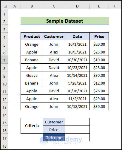
We take a data set that contains the product, customer, date, and sales of a Fruit Shop. For instance, we will apply 5 different methods using SUMIFS. Before that add criteria and outcome cells in the data set.
This section provides extensive details on these methods. So, you should learn and apply these to improve your thinking capability and Excel knowledge. Hence, go through the methods below. We use the Microsoft Office 365 version here, but you can utilize any other version according to your preference.
1. SUMIFS with Comparison Operators and Multiple Criteria Along Two Columns
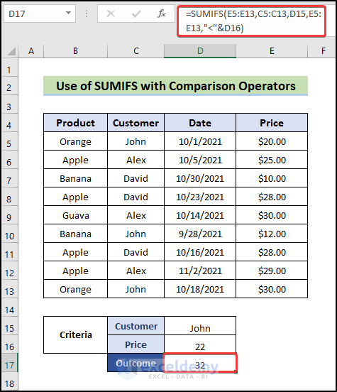
From our data set, we want to know the sum of sales to John that are less than 22 dollars. Here, the 1st criterion is the amount sold to John and 2nd one is the price is less than 22 dollars. Now, set these two criteria in the sheet. Inputs are John in the Customer box and 22 in the Price box. Therefore, follow the below steps to perform the task.
Steps:
- First, go to Cell D17.
- Next, write down the SUMIFS function.
- In the 1st argument select the range E5:E13, which value we want.
- In the 2nd argument select the range C5:C13 and select Cell D15 as the 1st criterion for John.
- Add 2nd criteria of range E5:E13 that contains the price. Then select smaller than sign and Cell D16. The formula becomes:
=SUMIFS(E5:E13,C5:C13,D15,E5:E13,"<"&D16)- Next, press Enter.
- Consequently, this outcome is the total sales to John less than 22 dollars each.
Read More: How to Apply SUMIFS with Multiple Criteria in Different Columns
2. Use SUMIFS in Excel with Date Criteria in Column
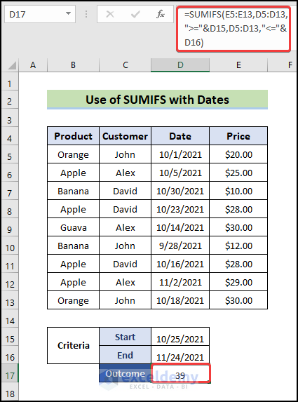
Here we will find sales compared to date. Let’s calculate the sales for the last 30 days. We will count today to the last 30 days. So, learn the below process.
Steps:
- First, we will set the start and end dates.
- Next, go to cell D17.
- Then, write down the SUMIFS.
- In the 1st argument select the range E5:E13, which indicates the price.
- After that, in the 2nd argument select the range D5:D13 that contains the date and input greater than equal sign and select cell D15 as the starting date.
- Add other criteria that are less than equal in the same range and select cell D16 as the ending date. So, the formula becomes:
=SUMIFS(E5:E13,C5:C13,D15,E5:E13,"<"&D16)- Then, press Enter.
- Consequently, this is the sales amount for the last 30 days.
- Hence, we can do this for any specific date or date range.
Read More: Excel SUMIFS with Multiple Vertical and Horizontal Criteria
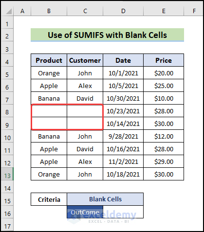
3. Excel SUMIFS with Blank Rows Criteria
We can make a report of blank cells by the SUMIFS function. For this, we need to modify our data set. Then, remove elements from the Product and Customer column, so that we can apply the function with some criteria. So, the data set will look like this. Therefore, follow the below steps.
Steps:
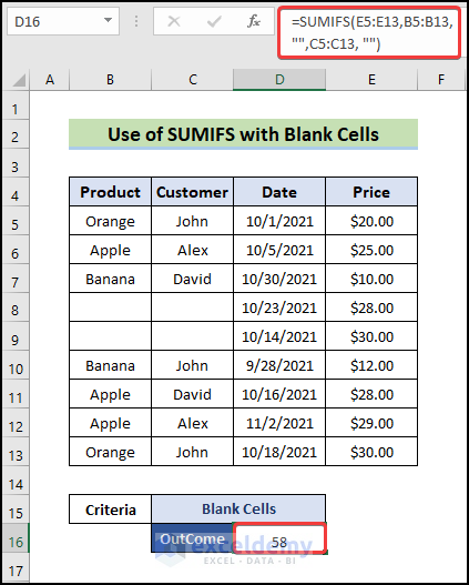
- First, go to cell D16.
- Then, write down the SUMIFS.
- After that, in the 1st argument select the range E5:E13, which indicates price.
- In the 2nd argument select the range B5:B13 and check blank cells.
- Add other criteria and that range is C5:C13. If both the columns alongside cells are blank then it will show an output. So, the formula becomes:
=SUMIFS(E5:E13,B5:B13, "",C5:C13, "")- Now, press Enter.
- Here, we will see that 2 cells of each column are blank. And the outcome is the sum of them.
4. SUMIFS with Non-Blank Cells Criteria Along Column & Row
We can get by in two ways. Using the SUM with SUMIFS function and only the SUMIFS function. Therefore, learn the below steps.
4.1 Using SUM-SUMIFS Combination
We can easily get this with the help of method 3.
Steps:
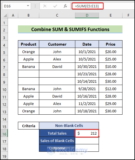
- First, add 3 cells in the datasheet to find our desired outcome.
- Then, get the total sales of Column E in cell D16.
- Afterward, Write the SUM function and the formula will be:
=SUM(E5:E13)- Now, press Enter.
- After that, in the D17 cell write down the formula of sales of blank cells that we get in the previous method. The formula will look like this:
=SUMIFS(E5:E13,B5:B13,"",C5:C13,"")- Again, press the Enter button.
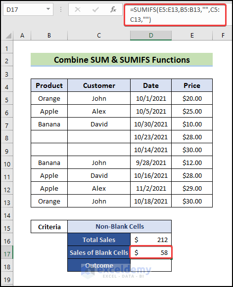
- Now, subtract these blank cells from the total sales in the D18 cell. So, the formula will be:
=SUM(E5:E13)-SUMIFS(E5:E13,B5:B13,"",C5:C13,"")- Finally, press Enter.
- Consequently, the outcome is the total sales of non-blank cells.

4.2 Using SUMIFS Function Alone
We can also get the total of all non-blank cells using the SUMIFS function only. So, follow the below steps.
Steps:
- First, go to Cell D16
- Then, write down the SUMIFS
- In the 1st argument select the range E5:E13, which indicates the price.
- After that, in the 2nd argument select the range B5:B13 and check blank cells.
- Moreover, add other criteria and that range is C5:C13. If both the column’s same cell is non-blank, then it will show an output that is the sum. So, the formula becomes:
=SUMIFS(E5:E13, B5:B13, "<>",C5:C13, "<>")- Again, press Enter.
- Consequently, this is the output of all the non-blank cells.
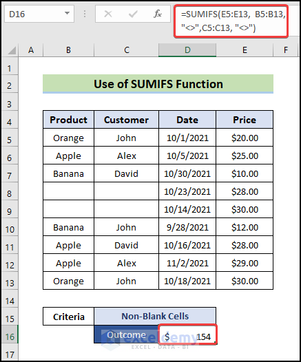
<> – It means not equal.
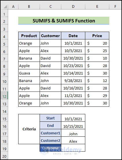
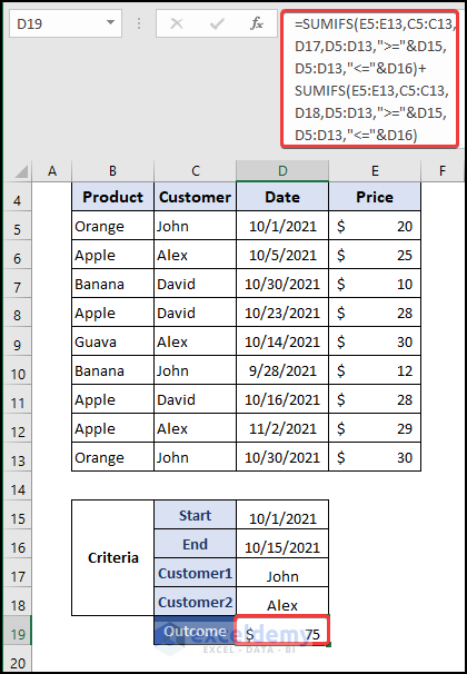
5. SUMIFS + SUMIFS for Multiple OR Criteria Along Column and Row
In this method, we want to apply multiple criteria multiple times. We used SUMIFS two times here to complete the task. First, we take John as a reference. Then, we want to find out the total sales to John between 1st October to 15th October. In the 2nd criterion take Alex as a reference for the same period. So, the data set will look like this:
- Firstly, go to Cell D19.
- Then, write down the SUMIFS function.
- After that, in the 1st argument select the range E5:E13, which indicates price.
- Subsequently, in the 2nd argument, select the range C5:C13 and select D17 as the reference customer.
- Then add the date criteria. So, the formula becomes:
=SUMIFS(E5:E13,C5:C13,D17,D5:D13,">="&D15,D5:D13,"<="&D16)+SUMIFS(E5:E13,C5:C13,D18,D5:D13,">="&D15,D5:D13,"<="&D16)- Again, press Enter.
- Finally, this is the sum of John and Alex in each period.
Read More: How to Use SUMIFS with Multiple Criteria in the Same Column
Excel SUMPRODUCT Function: Alternative to SUMIFS for Matching Multiple Criteria Along Column and Row
There are some alternative options through which we can achieve the same outputs. And in fact, they are a bit easier sometimes. Therefore, go through the following alternative methods.
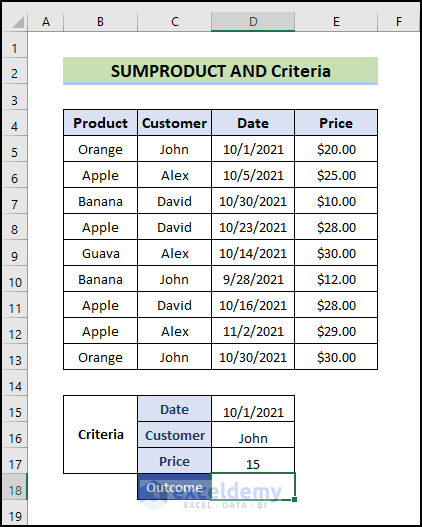
1. SUMPRODUCT with Multiple AND Criteria
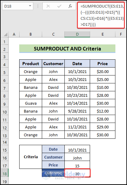
Here, we will apply the SUMPRODUCT function for AND type multiple criteria along with columns and rows. For instance, we will calculate the total products sold to John after 1st October which is higher than 15 dollars. SUMPRODUCT function will be used to make the solution easier. Modify the reference dataset a bit for this method.
Steps:
- First, go to cell D18.
- Then, write down the SUMPRODUCT Select range E5:E13 in the 1st argument which indicates the price. The formula becomes:
=SUMPRODUCT(E5:E13,(--(((D5:D13)>D15)*((C5:C13)=D16)*((E5:E13)>D17))))- After that, press Enter.
- See, we have got the result with less complication and using multiple criteria.
Read More: SUMIFS: Sum Range Across Multiple Columns
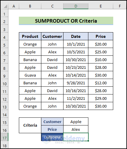
2. SUMPRODUCT with Multiple OR Criteria
Here, we will apply the SUMPRODUCT function for OR type multiple criteria along column and row. Here, we want to calculate the total sales of Apple and Alex. Moreover, it will include Apple and Alex both. Hence, we will do this by applying the SUMPRODUCT function. So, after modifying the data set will look like this:
Steps:
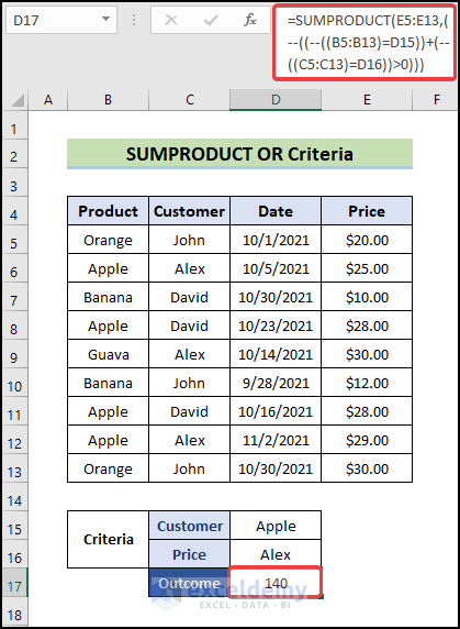
- First, go to cell D18
- Then, write down the SUMPRODUCT And the formula becomes:
=SUMPRODUCT(E5:E13,(--((--((B5:B13)=D15))+(--((C5:C13)=D16))>0)))- Now, press the Enter button.
- Finally, OR type multiple criteria can easily be solved in this way.
Download Practice Workbook
Download this practice workbook to exercise while you are reading this article.
Conclusion
In this article, we showed different ways to use the SUMIFS with multiple criteria along columns and rows. Moreover, we also attached alternative methods compared to SUMIFS. Hope this helps you get the exact solution. So, stay with us and provide your valuable suggestions. Keep learning new methods and keep growing!
Related Articles
- How to Apply SUMIFS with INDEX MATCH for Multiple Columns and Rows
- Exclude Multiple Criteria in Same Column with SUMIFS Function
- How to Use VBA SUMIFS with Multiple Criteria in Same Column
<< Go Back to Excel SUMIFS with Multiple Criteria | Excel SUMIFS Function | Excel Functions | Learn Excel
Get FREE Advanced Excel Exercises with Solutions!
