How to Sum Colored Cells in Excel (4 Ways)

There’re no built-in Excel functions that sum up the colored cells in Excel by themselves. Yet multiple ways can manage to sum up the cells based on their cell colors. In this blog post, you will learn 4 distinct ways, to sum up, the colored cells in Excel with easy examples and proper illustrations.

In the below image you will find an overview of the whole article.

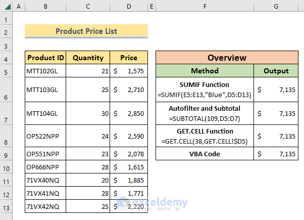
We will be using a Product Price List data table to demonstrate all the methods, to sum up, colored cells in Excel.

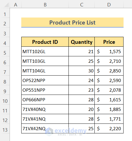
So, without having any further discussion let’s get into all the methods one by one.

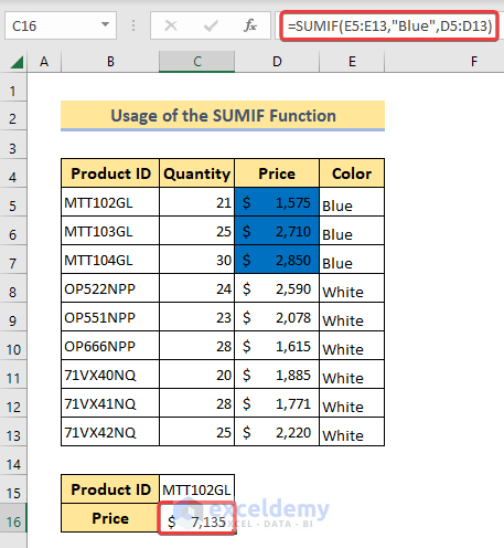
1. Using Excel SUMIF Function to Sum Colored Cells

Suppose, you want to sum up the total price of the products having “MTT” in their product ids. To mark those products, you have attributed them with blue color. Now, we will discuss a formula that will sum up the values of the cells indicated by blue color. To do so, we can use the SUMIF function. Now follow the steps below to see how to do it.

🔗 Steps:

❶ First of all, add an extra column to specify the cell colors in column “Price”.

❷ Then select cell C16 ▶ to store the formula result.

❸ After that type

❹ Finally press the ENTER button.

Read More: How to Sum Selected Cells in Excel (4 Easy Methods)

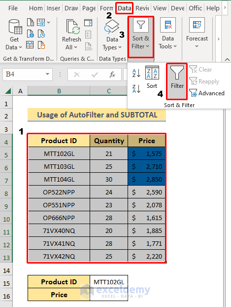
2. Using AutoFilter and SUBTOTAL to Add Colored Cells

We can use the AutoFilter feature and the SUBTOTAL function too, to sum the colored cells in Excel. Here are the steps to follow:

🔗 Steps:

❶ First of all, select the whole data table.

❷ Then go to the Data ribbon.

❸ After that, click on the Filter command.

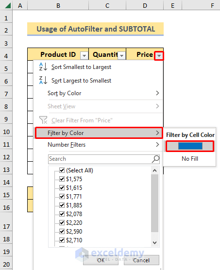
❹ Now click on the dropdown icon at the corner of the Price column header.

❺ Then from the dropdown menu select Filter by Color.

❻ Then click on the blue color rectangle.

❼ Now select cell C16 ▶ to store the formula result.

❽ Type

❾ Finally finish the whole process by pressing the ENTER button.

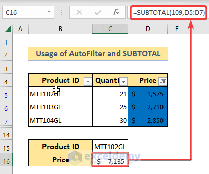
That’s it.

Read More: How to Sum Filtered Cells in Excel (5 Suitable Ways)

Similar Readings

• How to Sum by Group in Excel (4 Methods)
• [Fixed!] Excel SUM Formula Is Not Working and Returns 0 (3 Solutions)
• How to Sum Only Positive Numbers in Excel (4 Simple Ways)
• Sum by Font Color in Excel (2 Effective Ways)
• How to Sum Range of Cells in Row Using Excel VBA (6 Easy Methods)

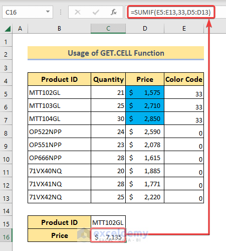
3. Using Excel GET.CELL Function to Sum Colored Cells

You can use the GET.CELL function along with the SUMIF function to sum up the colored cells in Excel. Now follow the steps below to see how to incorporate them together, to sum up, the colored cells.

🔗 Steps:

❶ First of all, go to Formulas ▶ Defined Names ▶ Name Manager.

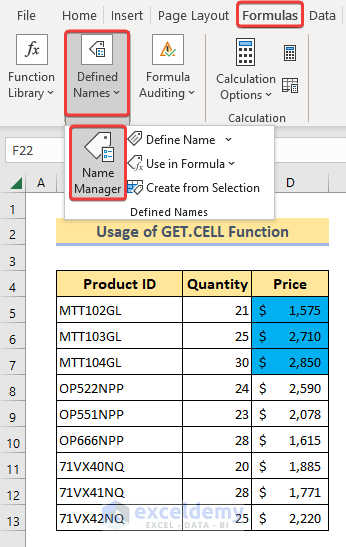
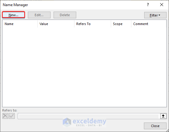
The Name Manager dialog box will pop up. From that box:

❷ Click on New.

After that, the Edit Name dialog box will pop up on the screen. From there,

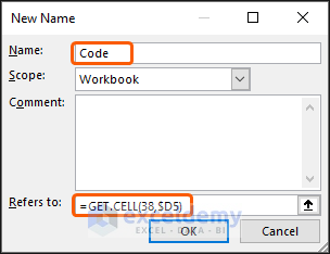
❸ Assign a name, for example, Code within the Name bar.

❹ Type the following code within the Refers to the bar.

❺ After that hit the OK button.

❻ Now you have to create a new column. For instance, the Code is as follows.

❼ Select cell E5 and type

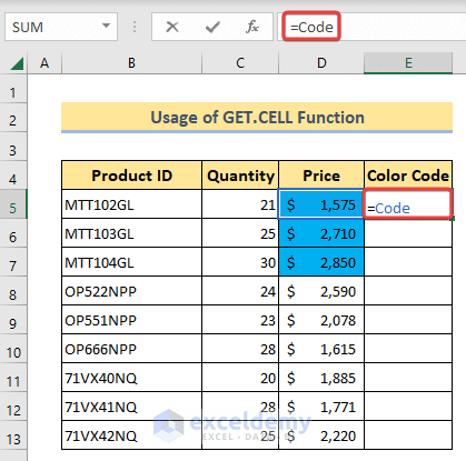
• Then, press the ENTER button.

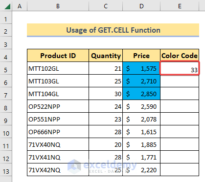
❽ Now drag the Fill Handle icon to the end of the Code column.

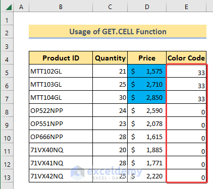
❾ Now select cell C16 and enter the formula:

❿ Finally, terminate the process by pressing the ENTER button.

So, here comes the result!

Read More: Sum to End of a Column in Excel (8 Handy Methods)

4. Using Excel VBA to Add Colored Cells

You can also sum up the colored cells by using the VBA code. In this section, we will be creating a user-defined function using VBA, to sum up, the colored cells.

Now follow the steps below:

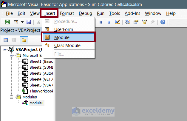
❶ First of all, press the ALT+F11 button to open the Excel VBA window.

❷ Now, go to the Insert ▶ Module.

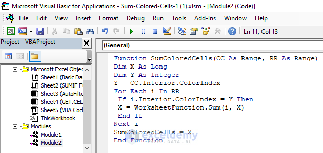
❸ After the copy the following VBA code.

Function SumColoredCells(CC As Range, RR As Range)
Dim X As Long
Dim Y As Integer
Y = CC.Interior.ColorIndex
For Each i In RR
 If i.Interior.ColorIndex = Y Then
 X = WorksheetFunction.Sum(i, X)
 End If
Next i
SumColoredCells = X
End Function

❹ Now paste and save this code in the VBA editor.

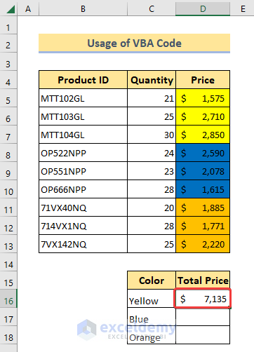
❺ Now select cell D16 ▶ to store the sum result.

❻ Enter the code within the cell:

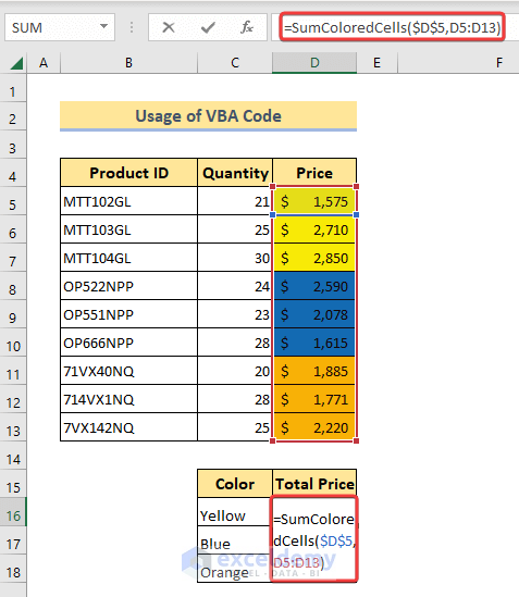
This code will sum up all the cells indicated by yellow color.

❼ Finally, hit the ENTER button.

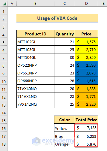
📓 Note:

• Formula to sum up the Blue painted cells:

Where cell $D$8 is a sample Blue painted cell.

• Formula to sum up the Orange painted cells:

Where cell $D$11 is a sample Orange painted cell.

Read More: Sum Cells in Excel: Continuous, Random, With Criteria, etc.

Things to Remember When Adding Colored Cells in Excel

📌 Be careful about the syntax of the functions.

📌 Insert the data ranges carefully into the formulas.

Download Practice Workbook

You are recommended to download the Excel file and practice along with it.

Conclusion

To wrap up, we have illustrated 4 different methods overall, to sum colored cells in Excel. Moreover, you can download the practice workbook attached along with this article and practice all the methods with that. And don’t hesitate to ask any questions in the comment section below. Surely we will try to respond to all the relevant queries asap.

Related Articles

• How to Sum Only Visible Cells in Excel (4 Quick Ways)
• Sum All Matches with VLOOKUP in Excel (3 Easy Ways)
• How to Calculate Sum of Squares in Excel (6 Quick Tricks)
• Sum If a Cell Contains Text in Excel (6 Suitable Formulas)
• How to Sum Multiple Rows in Excel (4 Quick Ways)