If your Excel worksheet contains full names in a column and you want to split the names into two columns, then you are in the right place. In this article, you will learn 5 quick ways to split names in Excel into two columns.
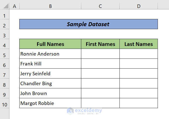
Let’s introduce our sample dataset first. In the column (B5:B10), we have our full names. Our goal is to split these names into the First Names and Last Names columns.
1. Using Convert Text to Columns Wizard to Split Names in Excel into Two Columns
The most common way to split the text into several columns is to use Convert Text to Columns Wizard. Just follow the steps below to apply this amazing trick.
Steps:
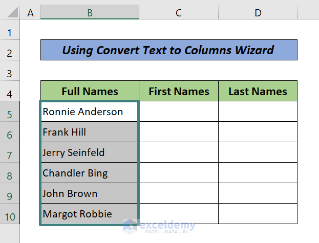
- Select the cells (B5:B10) that include the texts you need to split.
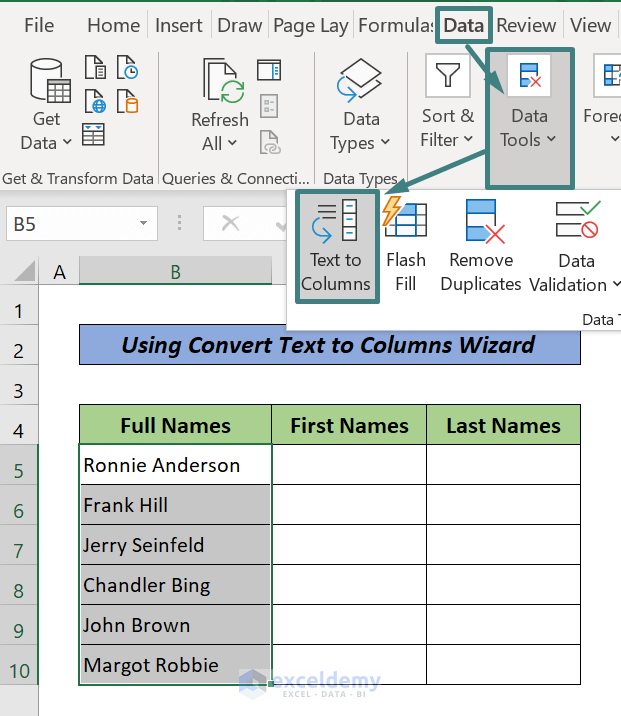
- Select Data > Data Tools > Text to Columns. The Convert Text to Columns Wizard window will appear.
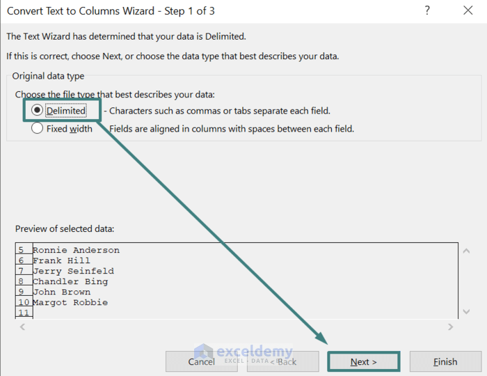
- Choose Delimited > click on Next.
- Choose the Delimiters for your texts. In this example, the delimiter is space. Then, click on Next.

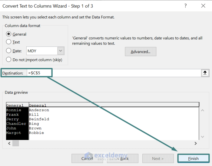
- Choose the Destination (C5) in the current worksheet where you want to split texts to display. Finally, click on Finish.
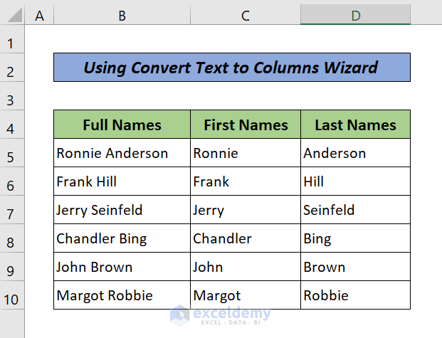
Here is the split data-
Read More: Separate First and Last Name with Space Using Excel Formula
2. Splitting Names into Two Columns Using Excel Flash Fill Feature
The Flash Fill can split your texts by identifying the pattern. Just follow the steps below to learn this magic trick.
Steps:
- In the neighboring cell C5, type the 1st name of the 1st full name. In the next-down cell C6, type the 1st name of the 2nd full name. Continue this activity until you see the Flash Fill show you a suggestion list of the 1st names in grey color.

- Press ENTER. You will see the rest of the cells with respective 1st names.

Repeat the steps for the last names of the full names.
Finally, here is the result,

Read More: How to Split Names Using Formula in Excel
3. Using Excel Formulas to Split Names into Two Columns
We can split a full name into first and last names by applying some built-in Excel formulas.
3.1. Getting First Name in First Column
Combining LEFT and FIND functions together helps us to split a full name separated by space into two columns. Just follow the steps below to do this.
Steps:
- First, write down the following formula in an empty cell C5.
=LEFT(B5, FIND(" ",B5)-1)Here, the FIND function gives the location of the first space from the string B5 and The LEFT function returns the characters from the string that is before the first space. You need to minus 1 to get the data excluding space.

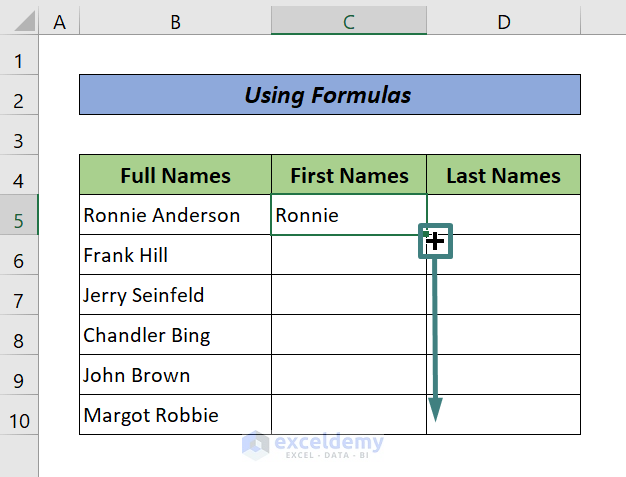
- Press ENTER. You will see the 1st name in Cell C5. Now, drag the Fill Handle to get the 1st names from the rest of the full names.
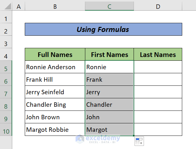
Finally, here is the result,
3.2. Getting Last Name in 2nd Column
Combining RIGHT and FIND functions together helps us to split a name separated by space into two columns. Just follow the steps below to do this.
Steps:
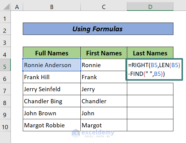
- First, write down the following formula in an empty cell D5.
=RIGHT(B5,LEN(B5)-FIND(" ",B5))Here, LEN(B5) determines the length of the string in cell B5.
The FIND(“ ”, B5) gives the location of the space from the full name and finally, the RIGHT function returns the characters from the full name which is after the space.
- Press ENTER. You will see the last name in Cell D5. Now, drag the Fill Handle to get the last names from the rest of the full names.
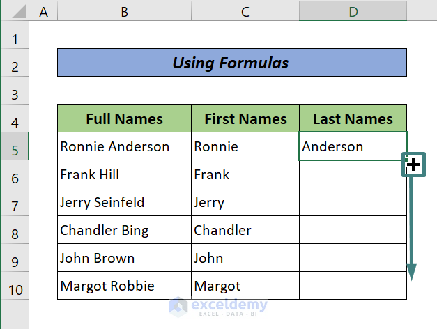
Finally, here is the result,

Read More: How to Separate First Name Middle Name and Last Name in Excel Using Formula
4. Splitting Names into Two Excel Columns Using Find & Replace Tool
If you love the flexibility that comes with Find and Replace in Excel, you can use this magical strategy.
4.1. Getting First Name in One Column
Just follow the steps below.
Steps:
- Copy all the full names, and paste them into the neighboring column (C5:C10) titled First Names.
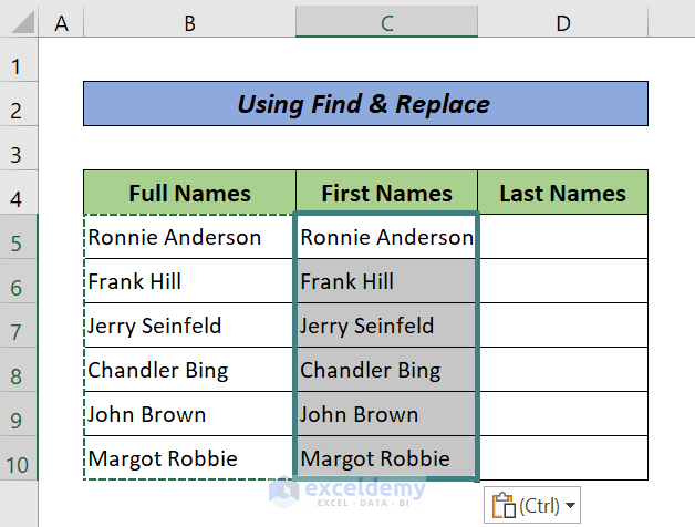
- Select C5:C10, go to the Home tab > Find & Select > Replace. A Find and Replace dialog box will pop up. Or just press the CTRL+H key.

- Enter “ *” ( 1 space before asterisk symbol) at Find what box and leave blank at Replace with box. Click on Replace All. Now, close the window.

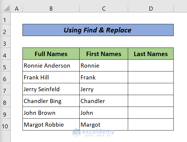
Here is the result,
4.2. Getting Last Name in Another Column
Just follow the steps below.
Steps:
- Copy all the full names, and paste them to the neighboring column (D5:D10) titled Last Names.
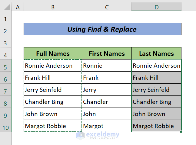
- Select D5:D10, go to the Home tab > Find & Select > Replace. A Find and Replace dialog box will pop up. Or just press the CTRL+H key.
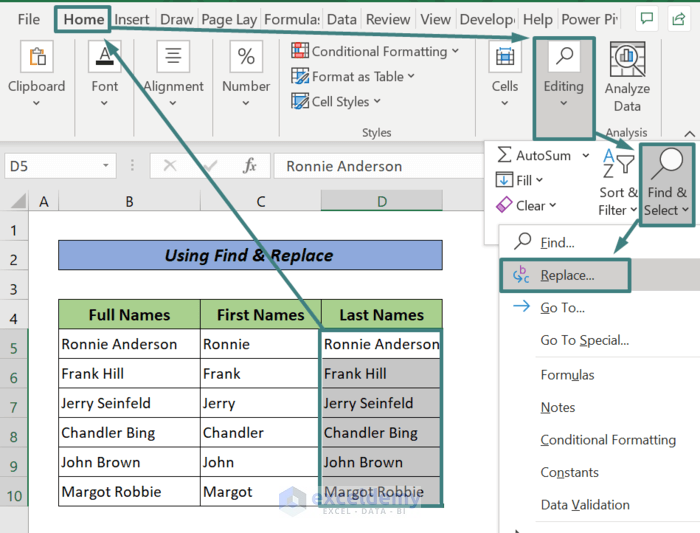
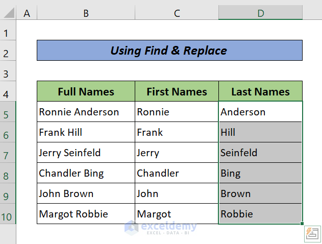
- Enter “* ” ( 1 space after asterisk symbol) at Find what box and leave blank at Replace with box. Click on Replace All. Now, close the window.

Here is the result,
Read More: Excel VBA: Split First Name and Last Name
Download Practice Workbook
Conclusion
In this tutorial, I have discussed 4 quick ways to split names in Excel into two columns. I hope you found this article helpful. Drop comments, suggestions, or queries if you have any in the comment section below.

