How to Split Data in Excel (5 Ways)

In different circumstances, we need to split our data into different pieces. These dissections of data are usually done by space, commas, or some other criteria. Splitting of these data can really help us to get what part of the data we need at a given time. 5 useful and easy methods of how to split data in Excel will be discussed in this article.

How to Split Data in Excel: 5 Ways

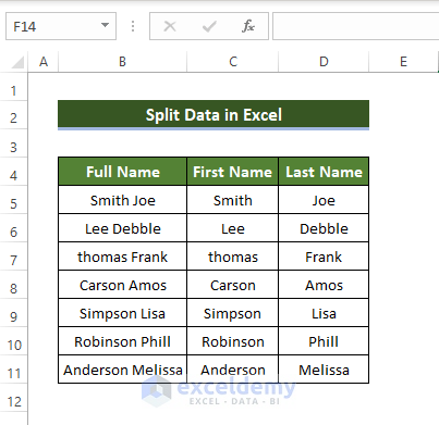
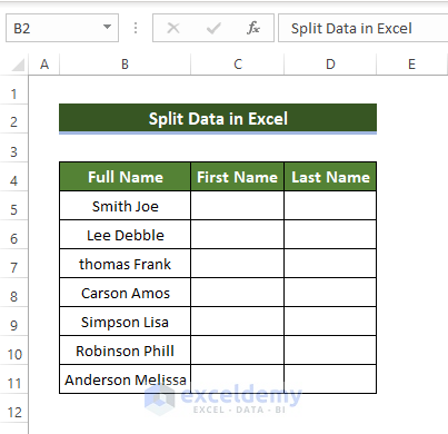
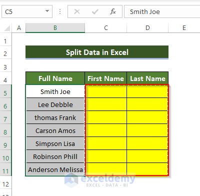
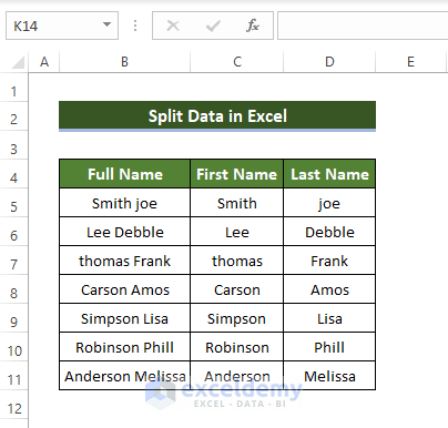
To demonstrate how to split data in Excel, we are going to use the following spreadsheet. The dataset contains the full names of different persons in the Full Name column, and their names first part and the second part.

1. Text to Columns Features to Split Data in Excel

In this process, delimiters like space, tab, and commas separate the selected data into one or more cells. The Text to Column feature is a great tool to split data in Excel.

Steps

• First, select all the cells that you wish to split.
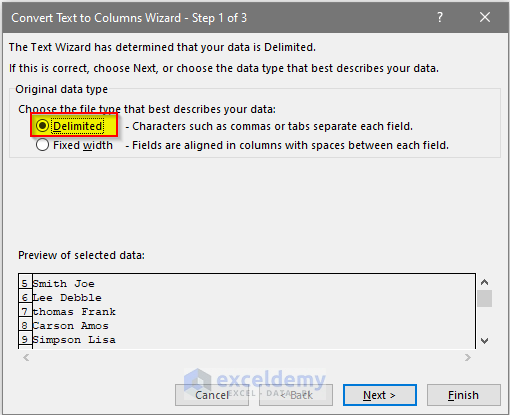
• Go to Data > Text to Columns.

• A new dialog box will open. From that box select delimited and click Next.

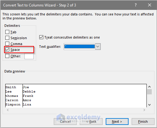
• After clicking Next, the next dialog box will appear.
• In that dialog box tick the Space option box, as we want to split the given data according to the position of space between words.

• Then in the next dialog box select General.
• Below the Column data format box, there is a cell reference box named Destination. In that box, you have to enter cell reference to present your split data.
• Click Finish in the dialog box, after selecting the destination cells.

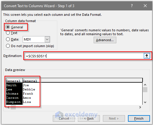
• Select your destination cells like below in the Destination box.

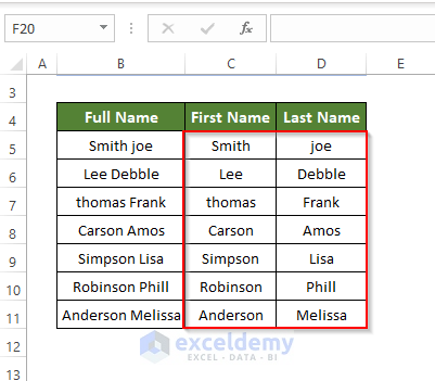
• After clicking Finish, you will notice that all of the names are now split into last and first names.

2. Split Cells in Excel Using Formulas

The formula can be a handy tool while splitting data in Excel. Using the TEXT function or TRIM/MID, we can easily and flexibly split different types of data.

2.1 Formula with the Text Functions

Steps:

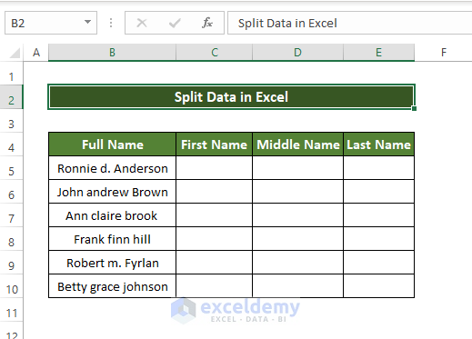
• We are going to use a different dataset for this method. This dataset contains a middle name column compared to the previous dataset.

• We enter the following formula in cell C5.

• We select the Fill Handle and drag it to cell C10.

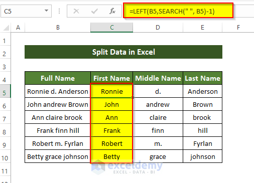
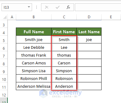
• This formula will split the first part of the Full Name column.
• To split the middle part of the First Name column, enter the following formula and press Enter.

• After pressing enter, split the middle part of the full name in cell D5.

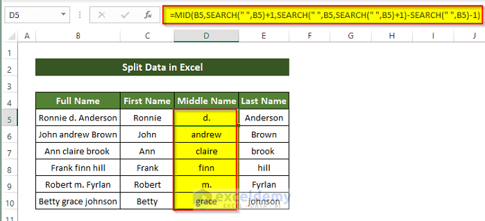
• After that, drag the fill handle button to cell D10. It will split the other Full Names middle part.
• To split the last part of the Full Name column, enter the following formula below.

• After pressing enter, you will see that the last part of the name in cell B5 is split into cell E5.

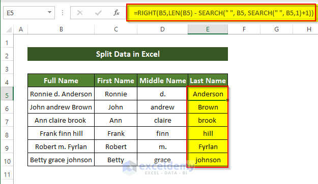
Drag the fill handle button to cell E10. It will split the other full name’s last part in the Last Name column.

2.2 Use of Trim and Mid Functions to Split Data

Steps:

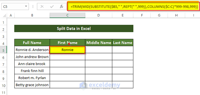
• First, you need to enter the following formula into cell C5.

• This formula will split the first part of the Full Name in the First Name column.

• After that, select the fill handle button, and drag it horizontally to cell E5.
• The Full Name column data in cell C5 will be completely split across three columns.

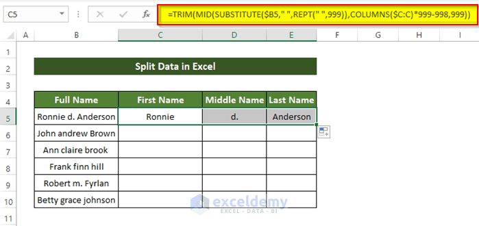
• Select range C5:E5, and drag the fill handle down to cell E10.

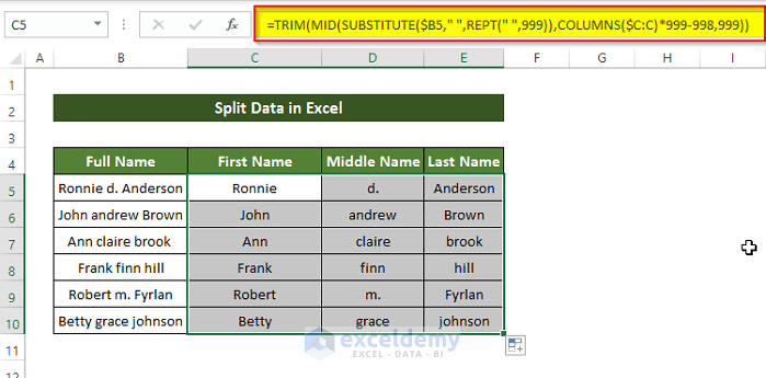
After releasing the fill handlebar, you will observe that all of your cell data are now split across three parts.

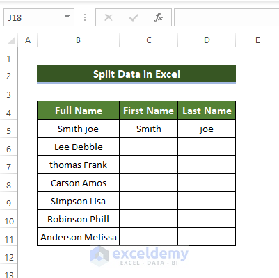
3. Split Data into Cells in Excel Using the Flash Fill Feature

Steps:

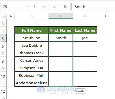
• At first, you need to fill up the first row of the dataset. That means you need to enter the split first name and last name in cells C5 and D5 respectively.

• Drag the corner handle to cell C11 by pressing right-click on the mouse.

• Then release the handle, upon releasing the handle, a new drop-down window will open.
• From that window, choose Flash Fill.

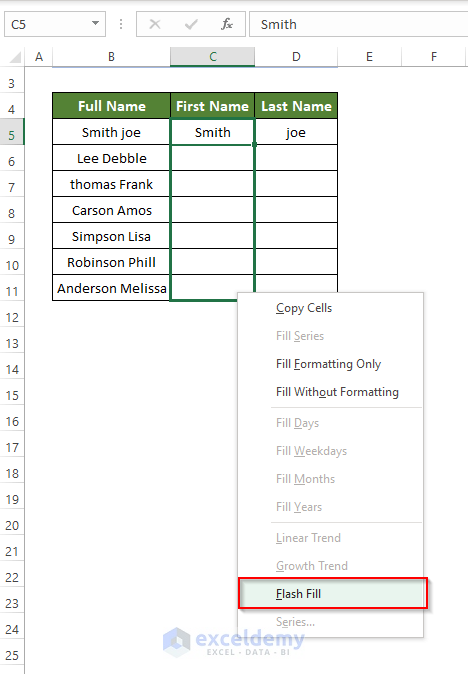
• Selecting the Flash Fill button will split the first part of the names in the name column as done in cell C5.

• Repeat the same process for the Last Name column, this will split the last part of the names in the Full Name column.

Now all the names in the Full Name column are split into two parts.

4. Split Cells and Text in Excel with Power Query

Using a powerful tool like Power Query in Excel, you can easily split the names in the Full Name column.

Steps:

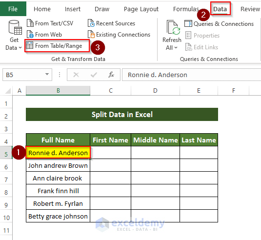
• Select any cell inside the table, and go to Data > From Table/Range.

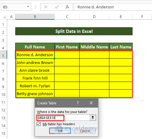
• Then a new window will appear named Create Table, in which you have to select the range of your table.

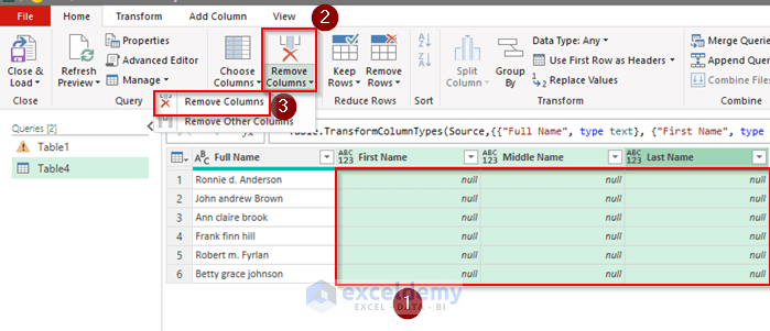
• After entering the range, a new window will open.
• From this window, you have to remove the empty columns.

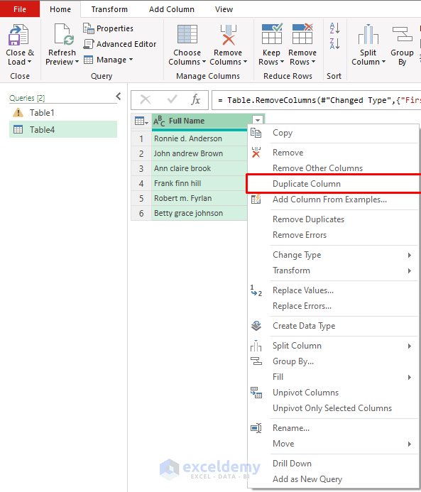
• After removing the columns, you need to duplicate the Full Name column.
• For that, right-click > Click on the Duplicate Column option from the menu.

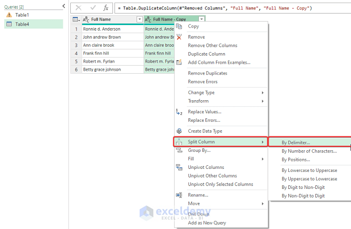
• Select Full Name – Copy column and right-click on the mouse.
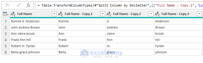
• From the Context Menu, go to Split Column > By Delimiter.

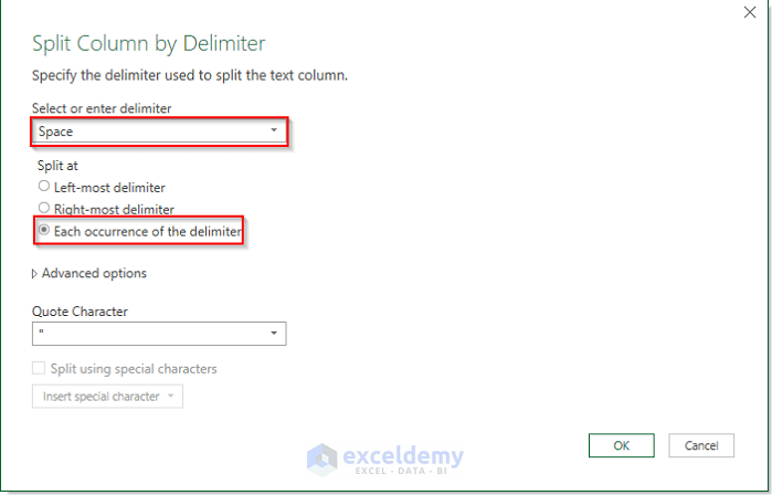
• A new window will open.
• In that window, select Space from the Select or enter delimiter section.
• Select Each occurrence of the delimiter at Split at and click OK.

• After clicking OK, you will see that full names have been split into three separate columns.

• Change those column names to First Name, Middle Name, and Last Name.
• Finally, click Close & Load.

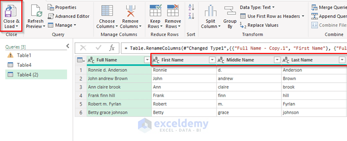
• After closing and loading the power tool, a new sheet will appear in the main workbook like this.

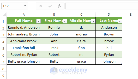
In this worksheet, you can clearly see that the names in the Full Name column are split into three separate parts based on the space between them.

5. Using VBA Macro to Split Data in Excel

A simple VBA code can solve all of the above problems quite easily. At the same time, the use of macros is quite hassle-free and time-saving.

Steps:

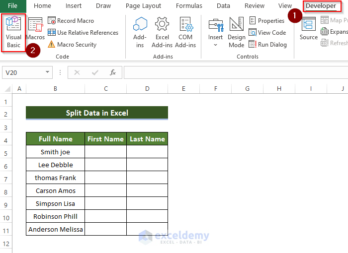
• Launch the Visual Basic editor from the Developer tab.
• Or press Alt + F11 on your keyboard.

• After launching the Visual Basic editor, a new window will launch.
• In the new window click Insert, then click Module.

• An Editor Window will open. In that editor, you need to write the following code.

Sub Split_Data()

Dim My_Array() As String, Column As Long, x As Variant

For m = 5 To 11
    My_Array = Split(Cells(m, 2), " ")
    Column = 3
    For Each x In My_Array
        Cells(m, Column) = x
        Column = Column + 1
    Next x
Next m

End Sub

• Upon writing the code, close the Module.
• From the View tab, click the Macros command, then select the View Macros option.

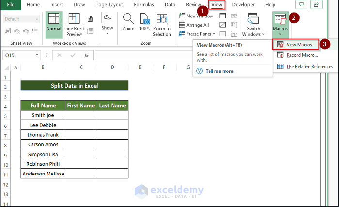
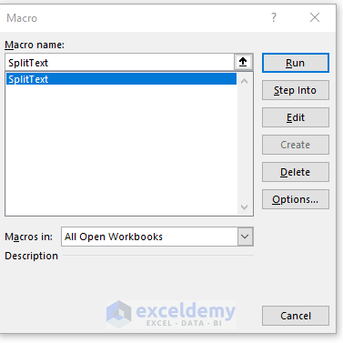
• Next, a new dialog box will open.
• From that dialog box, select the Macro that you just created and click Run.

• Upon clicking Run, you will see that all your names in the Full Name column are now split across three different parts.

Download Practice Workbook

Download this practice workbook.

Conclusion

To sum it up, the question of how to split data in Excel can be answered in 6 easy ways. They are mainly by using formulas, using the Text to Column feature, deploying Power Query and another one is to run a small VBA macro. The VBA process is less time-consuming and simplistic but requires prior VBA-related knowledge. Similarly, a power query is also a very convenient tool but a bit time-consuming.

On the other hand, other methods don’t have such a requirement. Text to Column method is by far the most convenient and easy to use among all of them. For this problem, a practice workbook is available to download where you can practice and get used to these methods.