Microsoft Excel is a ubiquitous tool for organizing and analyzing data. Oftentimes, we may need to separate numbers in Excel, therefore, knowing a couple of methods can save a lot of time and effort. This article demonstrates 5 useful ways how to separate numbers using formula in Excel. In addition, we’ll also explore how to split numbers and how to split numbers into two columns.
Watch Video – Separate Numbers Using Formula in Excel
How to Separate Numbers Using Formula in Excel: 5 Ways
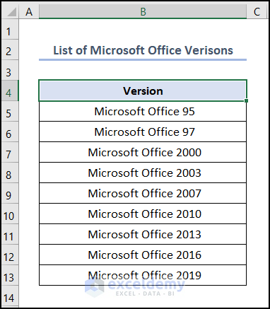
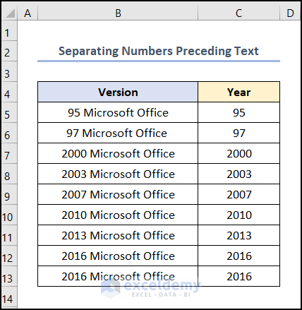
At this time, consider the List of Microsoft Office Versions dataset shown in the B4:B13 cells, which shows the different Versions of Microsoft Office starting from 1995 to 2019. Here, we want to extract only numbers from each cell, hence, let’s observe and learn about each method in detail.
Here, we have used the Microsoft Excel 365 version, you may use any other version according to your convenience.
Method 1: Using Combined Excel Formula
For one thing, functions are the heart and soul of Excel, and here we’ll combine various functions to extract only the numbers from each of the cells. So, let’s begin.
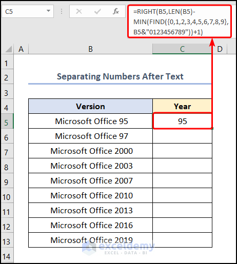
1.1 Separate Numbers After Text
First and foremost, the FIND function searches for the numbers within the given array, and the MIN function returns the smallest number from the given array. Additionally, the LEN function returns the total length of the string of text, and subtracting the position of the number from the total length tells the RIGHT function to separate numbers using the Excel formula.
📌 Steps:
- At the very beginning, go to the C5 cell >> enter the formula given below.
=RIGHT(B5,LEN(B5)-MIN(FIND({0,1,2,3,4,5,6,7,8,9},B5&"0123456789"))+1)
Here, the B5 cell refers to the text Microsoft Office 95.
Formula Breakdown:
- FIND({0,1,2,3,4,5,6,7,8,9},B5&”0123456789″) → returns the starting position of one text string within another text string. Here, {0,1,2,3,4,5,6,7,8,9} is the find_text argument while B5&”0123456789″ is the within_text argument. Here, the FIND function returns the position of the numeric values in the string of text.
- MIN(FIND({0,1,2,3,4,5,6,7,8,9},B5&”0123456789″)) → returns the smallest number in a set of values. In this case, the FIND({0,1,2,3,4,5,6,7,8,9},B5&”0123456789″) is the number_1 argument and the MIN function returns the smallest value within this array.
- Output → 18
- LEN(B5) → returns the number of characters in a string of text. Here, the B5 cell is the text argument which yields the value 19.
- Output → 19
- LEN(B5)-MIN(FIND({0,1,2,3,4,5,6,7,8,9},B5&”0123456789″))+1 → becomes
- 19 – 18 + 1 → 2
- RIGHT(B5,LEN(B5)-MIN(FIND({0,1,2,3,4,5,6,7,8,9},B5&”0123456789″))+1) → becomes
- RIGHT(B5,2) → returns the specified number of characters from the end of a string. Here, the B5 cell is the text argument whereas 2 is the num_chars argument such that the function returns the 2 characters from the right side.
- Output → 95
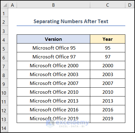
- Then, use the Fill Handle Tool to copy the formula into the cells below.
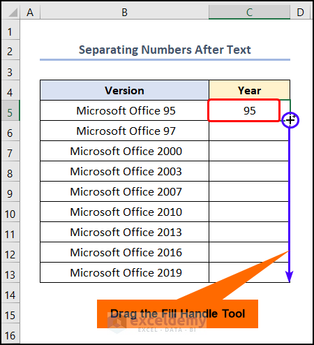
Lastly, the results should look like the image given below.
1.2 Separate Numbers Preceding Text
Alternatively, we can also utilize the SUBSTITUTE function to replace the existing text with new text and the LEN function to determine its length and the total length of the text string. Following this, apply the SUM function to calculate the total of the numeric values, which provides the number of characters for the LEFT function to separate numbers using the Excel formula.
📌 Steps:
- Initially, move to the C5 cell >> type in the expression given below.
=LEFT(B5,SUM(LEN(B5)-LEN(SUBSTITUTE(B5,{"0","1","2","3","4","5","6","7","8","9"},""))))
In this expression, the B5 cell indicates the text 95 Microsoft Office.
Formula Breakdown:
- SUBSTITUTE(B5,{“0″,”1″,”2″,”3″,”4″,”5″,”6″,”7″,”8″,”9″},””) → replaces existing text with new text in a text string. Here, the B5 refers to the text argument while Next, the {“0″,”1″,”2″,”3″,”4″,”5″,”6″,”7″,”8″,”9”} represents the old_text argument, and the “” points to the new_text argument which is left blank.
- LEN(SUBSTITUTE(B5,{“0″,”1″,”2″,”3″,”4″,”5″,”6″,”7″,”8″,”9″},””)) → returns the number of characters in the string of text. Here, the output from the SUBSTITUTE function is the text argument.
- SUM(LEN(B5)-LEN(SUBSTITUTE(B5,{“0″,”1″,”2″,”3″,”4″,”5″,”6″,”7″,”8″,”9″},””))) → adds all the numbers in a range of cells. Here, the SUM function returns the total of the numeric values.
- Output → 2
- LEFT(B5,SUM(LEN(B5)-LEN(SUBSTITUTE(B5,{“0″,”1″,”2″,”3″,”4″,”5″,”6″,”7″,”8″,”9″},””)))) → becomes
- LEFT(B5,2) → returns the specified number of characters from the start of a string. Here, the B5 cell is the text argument whereas 2 is the num_chars argument such that the function returns the 2 characters from the left side.
- Output → 95

Finally, your output should look like the picture given below.
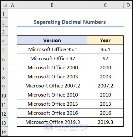
1.3 Separate Decimal Numbers
In a similar fashion, we can also separate decimal numbers using Excel formulas. Now, the process is remarkably similar to the previous method, so, just follow along.
📌 Steps:
- In the first place, insert the following equation into the C5 cell.
=RIGHT(B5,LEN(B5)-MIN(FIND({0,1,2,3,4,5,6,7,8,9},B5&"0123456789"))+1)
In this case, the B5 cell represents the text value of Microsoft Office 95.1.
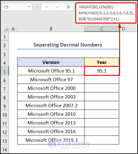
Eventually, after completing the above step, the output should look like the screenshot given below.
Method 2: Utilizing Flash Fill Feature
If using complex formulas doesn’t suit you then our next method might be the answer you’re looking for. Here, we’ll apply the Flash Fill feature of Excel to quickly separate the numbers from the text.
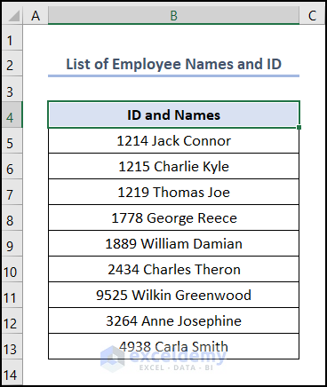
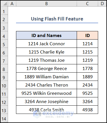
Suppose we have the List of Employee Names and ID dataset shown in the B4:B13 cells which contain the ID and Names. In this case, we want to separate the ID number and the First and Last Names respectively. So, just follow the steps shown below.
📌 Steps:
- In the first place, manually type in the first ID number which is 1214 in the C5 cell so that Excel can recognize a pattern.
- Next, navigate to the C6 and enter the first two digits of 1215 and Excel will show a preview of the autofill results >> hit the ENTER key.
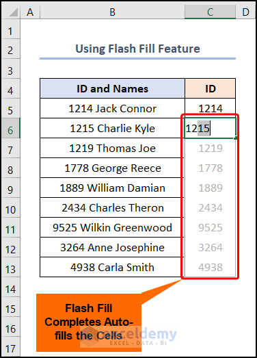
Subsequently, the results should look like the image given below.
Method 3: Employing Text to Columns Feature
Undoubtedly, Excel’s Text to Column feature becomes handy when separating numbers in one cell across multiple cells. Typically, there are two ways to apply the Text to Column feature, so let’s see how each of the techniques works.
3.1 Applying Delimiters Option
The delimiter option can split text data into separate columns based on space, tab, semicolon, etc. characters present within the text.
📌 Steps:
- First, select the B5:B13 cells >> proceed to the Data tab >> click the Text to Columns option.
For instance, the B5:B13 cells point to the ID and Names columns.
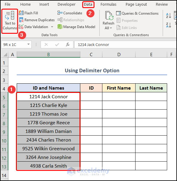
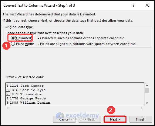
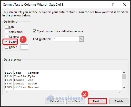
Now, this opens the Convert Text to Columns wizard.
- Second, choose the Delimited option >> hit the Next button.
- Third, insert a check mark for the Space delimiter >> press the Next button.
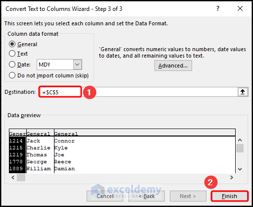
- Fourth, enter a Destination cell according to your preference, here it is the C5 cell >> click the Finish button.
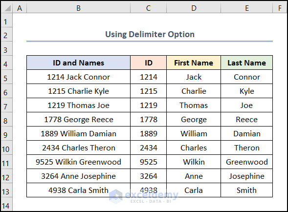
Consequently, the results should appear in the picture shown below.
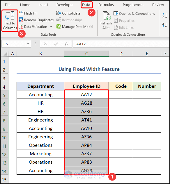
3.2 Utilizing Fixed Width Feature
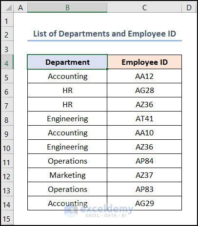
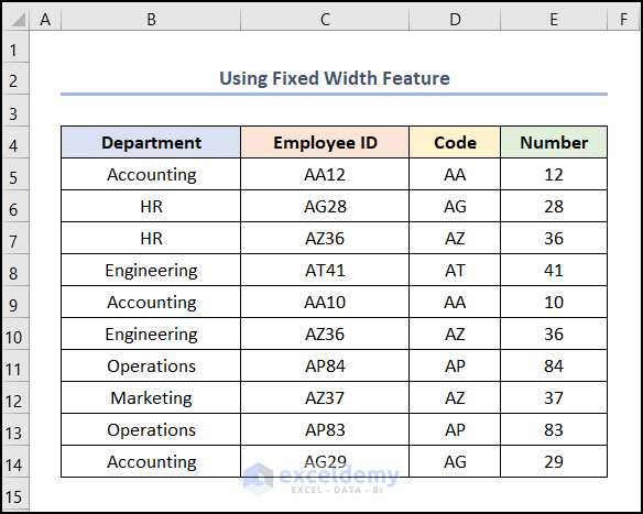
On this occasion, let’s consider the List of Departments and Employee ID dataset shown in the B4:C14 cells, which contain the Department and Employee ID respectively. In this situation, we want to separate the Employee ID into the Code and Number, since all the ID numbers consist of 2 digits. The Fixed Width option is the perfect candidate for this job.
📌 Steps:
- To begin with, select the C5:C14 cells >> jump to the Data tab >> press the Text to Columns option.
Specifically, the C5:C14 cells point to the Employee ID column.
In an instant, the Convert Text to Columns wizard pops out.
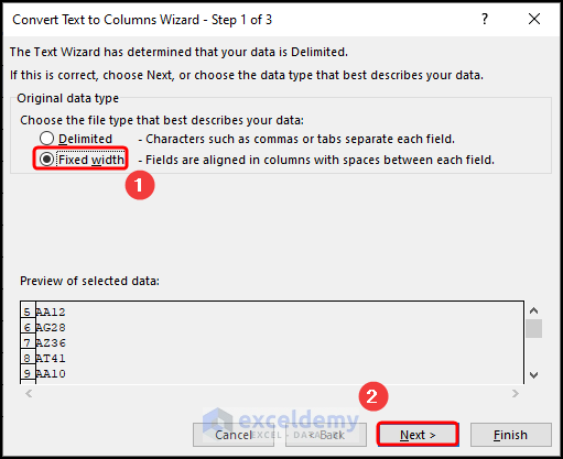
- Not long after, select the Fixed Width option >> press the Next button.
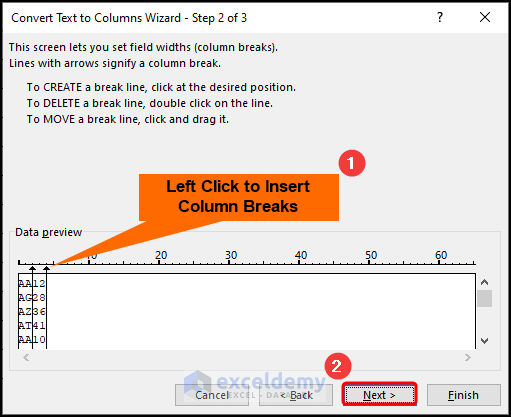
- In turn, Left click to insert column breaks after the Code and ID >> click the Next button.
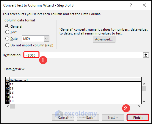
- Next, select the Destination cell, for example, the D5 cell >> hit the Finish button.
Ultimately, the end result should look like the screenshot provided below.
Method 4: Using Power Query Editor
Power Query is an often overlooked feature of Excel, despite its ability to organize and analyze data quickly and efficiently. In the following section, we’ll discuss how we can separate numbers in Excel with just a few clicks. So, let’s see it in action.
📌 Steps:
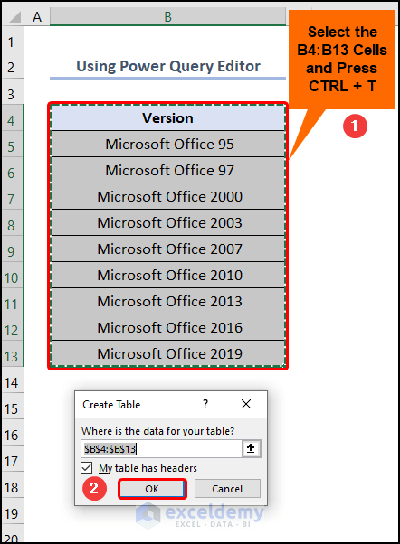
- To start with, select the B4:B13 cells >> hit the keyboard shortcut CTRL + T to insert an Excel Table >> press OK.
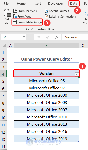
- Next, go to the B4 cell >> in the Data tab, click the From Table/Range option.
Not long after, the Power Query Editor window appears.
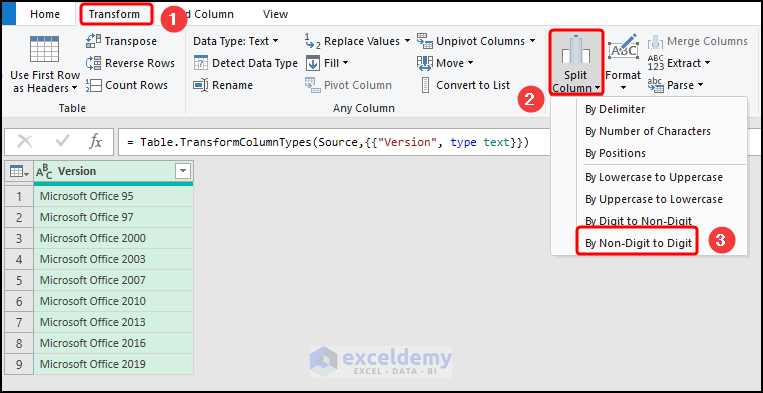
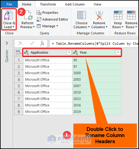
- From this point, move to the Transform tab >> press the Split Column drop-down >> choose the By Non-Digit to Digit option.
- Following this, Double-click the column headers to rename them >> press the Close & Load option to exit the Power Query window.
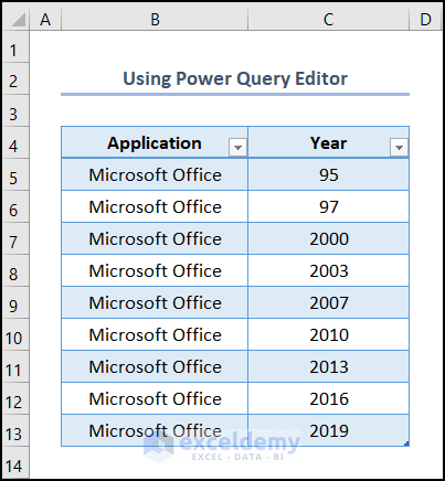
Finally, the output should look like the image depicted below.
Method 5: Applying VBA Code
If you often need to separate numbers using the Excel formula, then you may consider the VBA Code below. It’s simple and easy; just follow along.
📌 Steps:
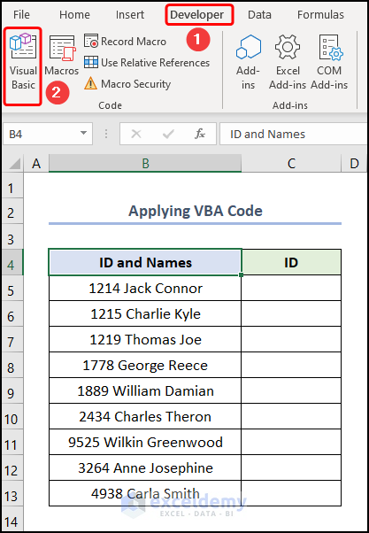
- First, navigate to the Developer tab >> click the Visual Basic button.
Now, this opens the Visual Basic Editor in a new window.
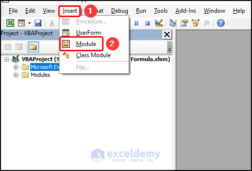
- Second, go to the Insert tab >> select Module.
For your ease of reference, you can copy the code from here and paste it into the window as shown below.
Function SplitNumAndText(str As String, op As Boolean)
num = ""
   txt = ""
   For i = 1 To Len(str)
       If IsNumeric(Mid(str, i, 1)) Then
            num = num & Mid(str, i, 1)
Else
            txt = txt & Mid(str, i, 1)
     End If
    Next i
If op = True Then
    SplitNumAndText = num
Else
    SplitNumAndText = txt
End If
End Function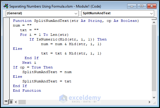
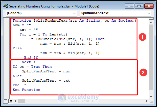
⚡ Code Breakdown:
Now, I will explain the VBA code used to separate numbers. In this case, the code is divided into 2 steps.
- In the first portion, declare the function SplitNumAndText where the first argument is a string and the second argument a Boolean type.
- Next, iterate through the whole string using For loop and If statement to check if the value is a number or not.
- In the later portion, use a second If statement to return output (Number or Text) based on the second argument. Simply put, passing 0 as the second argument will extract the Text while passing 1 returns the Number from the given string.
- Third, close the VBA window >> navigate to the C5 cell >> insert the function below.
=SplitNumAndText(B5,1)
Here, the B5 cell refers to the ID and Names value of 1214 John Connor.
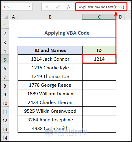
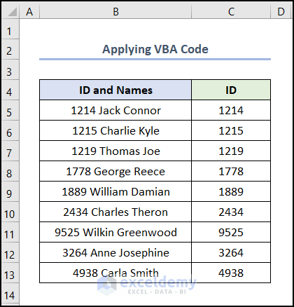
Ultimately, this should yield the results shown in the screenshot below.
How to Split Numbers Using Formula in Excel
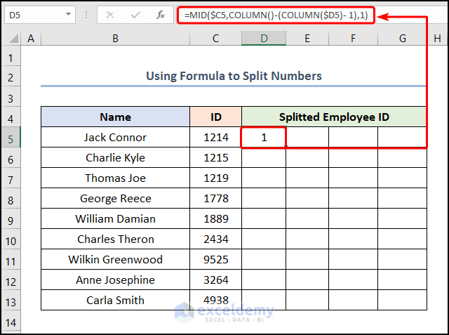
Another common scenario involves splitting numbers using a formula. Now, this can be done by combining the MID and COLUMN functions. Here, the MID function returns the characters from the middle of a text string while the COLUMN function provides the cell reference of the text string.
📌 Steps:
- Initially, jump to the D5 cell >> insert the expression into the Formula Bar.
=MID($C5,COLUMN()-(COLUMN($D5)- 1),1)
In the above expression, the C5 cell indicate the ID number 1214.
Formula Breakdown:
- COLUMN()-(COLUMN($D5)- 1) → returns the column number of a cell reference.
- 4 – (4-1) → 1
- MID($C5,COLUMN()-(COLUMN($D5)- 1),1) → becomes
- MID($C5,1,1) → returns the characters from the middle of a text string, given the starting position and length. Here, the C5 cell is the text argument, 1 is the start_num argument, and 1 is the num_chars argument such that the function returns the first character from the left side.
- Output → 1
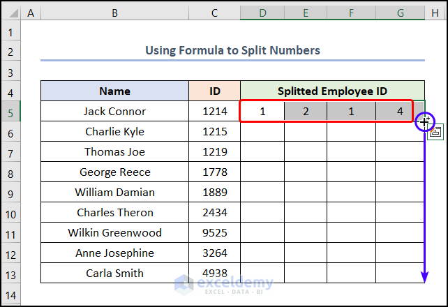
- Next, drag the Fill Handle tool across the rows to insert the remaining numbers.
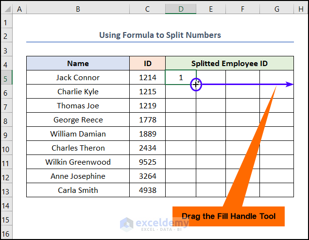
- In turn, select the D5:G5 cells and again use the Fill Handle tool to complete the table.
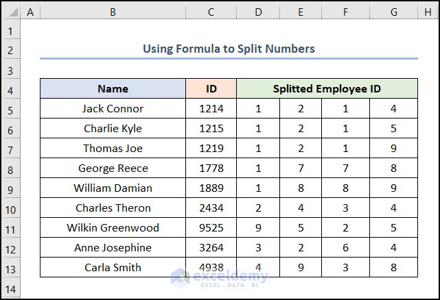
Eventually, the final output should look like the following screenshot.
How to Split Numbers into Two Columns in Excel
What if you want to split numbers into two columns? Then, you’re in luck since the next section provides the answer to your question. Now, allow us to demonstrate the process in the steps below.
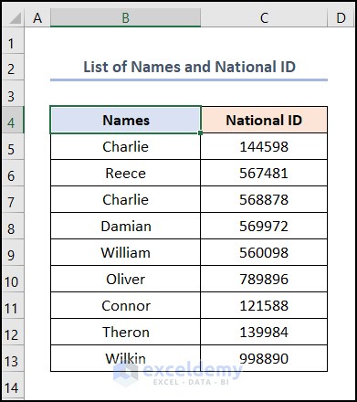
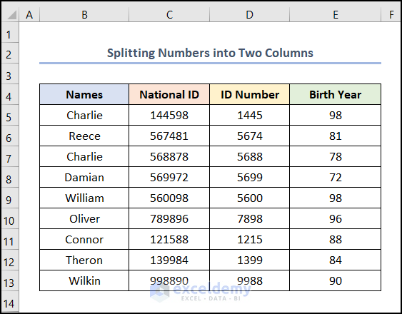
For instance, assume the List of Names and National ID dataset shown in the B4:C13 cells contains the Name and National ID numbers of a group of people. Admittedly, the last two digits of the National ID number represent the Birth Year of each person, and we want to split the first 4 and the last 2 digits into two separate columns.
📌 Steps:
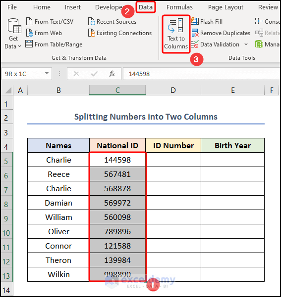
- In the first place, select the C5:C13 cells >> navigate to the Data tab >> click the Text to Columns option.
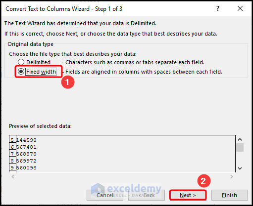
- Later, select the Fixed Width option >> press the Next button.
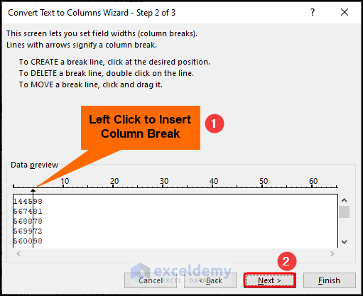
- Afterward, Left click to insert column breaks after the Birth Year >> click the Next button.
- In turn, select the Destination cell, like the D5 cell >> hit the Finish button.
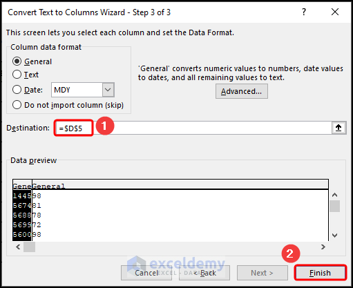
Subsequently, your results should look like the image shown below.
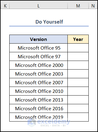
Practice Section
We have provided a Practice section on the right side of each sheet so you can practice yourself. Please make sure to do it by yourself.
Conclusion
In essence, this article shows 5 effective methods on how to separate numbers using formula in Excel. So, read the full article carefully and download the free workbook to practice. Now, we hope you find this article helpful and if you have any further queries or recommendations, please feel free to comment here.
<< Go Back to Separate Numbers Text | Split | Learn Excel
Get FREE Advanced Excel Exercises with Solutions!

Hi,
Good day!
I tried to use column to text method to separate a range of numbers in a cell(A1) and it works well on B1,C1,D1… But if I change the range of numbers in A1 again, the rest of the column does not change. May I know why? How can I have the rest of the column refresh with new numbers when I change the range of numbers in A1
Hello Edmund Goh,
Thank you for sharing your problem with us. I assume you have properly gone through the steps to separate numbers with the Text to Columns feature. The reason that any changes are not updating is because the Text to Columns feature is static and it will not take any changes from the source cell. Yes, this is a limitation of this feature. You will also face the same if you apply the Flash Fill feature. In this case, I will suggest you to apply any other methods from this article except Method 4 and 5. Then you will be able to get changes on the separated numbers from the text.
Let us know if it helps you.
Thank you.
Regards,
Guria
ExcelDemy.