How to Select Specific Data in Excel (6 Easy Methods)

Undoubtedly Microsoft Excel helps us to do our work easily. Seeking a large Excel Spreadsheet is not always easy. In this article, I’ll show you 6 methods by which you can easily select specific data in Excel based on their values under different conditions.

Below we presented a process where we used the VLOOKUP function to determine and extract the marks of the students.

How to Select Specific Data in Excel: 6 Easy Methods

Suppose, we have a datasheet where ID, Marks, and Student Names are given in Column B, column D, and Column C respectively. We will have to select some specific data using these values. In this section, we will discuss six easy methods to do it. In order to avoid any kind of compatibility issues please try to use the Excel 365 edition.

1. Find and Replace Tool to Select Specific Data in Excel

We can use the Find and Replace window to find and then select specific data. Below, are two separate methods to launch this Find and Replace window, using a Keyboard Shortcut and Using the Find and Replace command.

1.1 Using the Keyboard Shortcuts to Select Specific Data in Excel

Like other Keyboard shortcut methods, this is the easiest way to select specific data in Microsoft Excel. To quickly select specific data in Excel, execute the following steps.
Steps:
● At first on the keyboard press the Ctrl + F button.

• After that, the Find & Replace dialog box will appear.

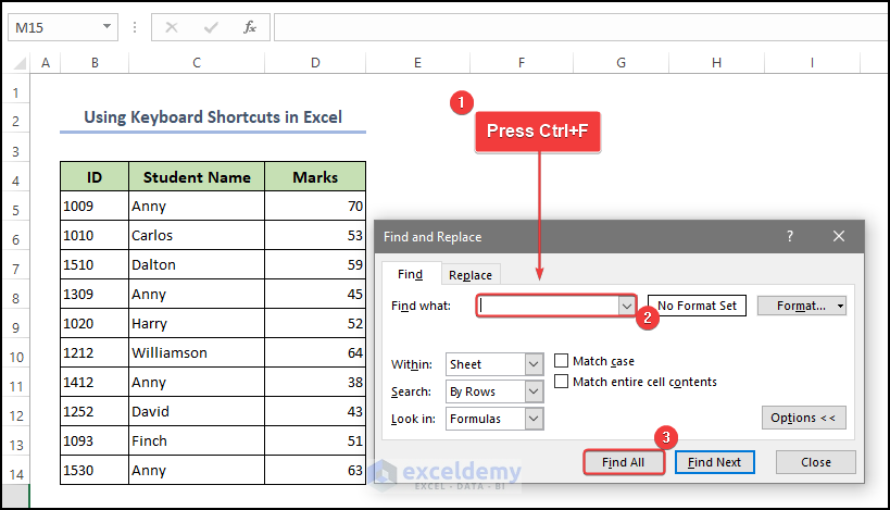
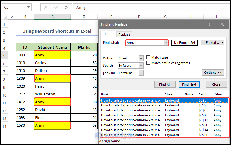
• Finally in the Find What text box insert the specific data that you want and click on Find All Then you will see the cells that have a character named Anny. They are also highlighted in the source data table.

1.2. Use of the Find Command to Select Specific Data in Excel

Suppose,  in our dataset, we want to find out the specific student name. Let’s follow the following steps to find out the name of that student.
Steps:
● At first go to Home > Editing > Find & Replace.

• Then select Find after this.

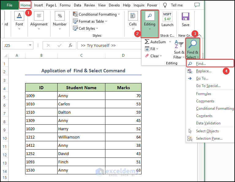
• After that, the Find & Replace dialog box will appear.
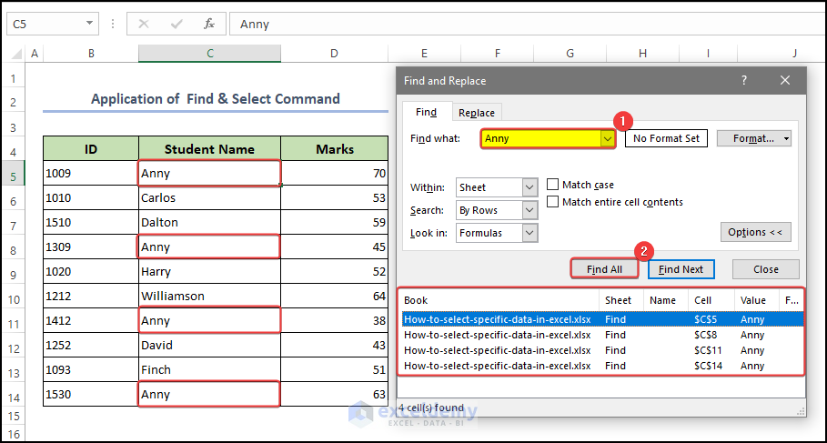
• Finally, in the Find text box enter the name of the student you want to find out and click on Find All Now, you will get your desired output in the spreadsheet cell. And you can select the specific data in Excel.

2. Apply the Lookup Functions to Select Specific Data in Excel

In MS Excel you can easily find specific data by using the LOOKUP function. Looking through a single column or row to find a particular value from the same place in a second column or row is the application of the LOOKUP Function. There are, however, two types of LOOKUP Functions and they are-
● The VLOOKUP Function
● The HLOOKUP Function
We will learn both of the functions in this section and how we can select the specific data in Excel.

2.1. Insert the VLOOKUP Function

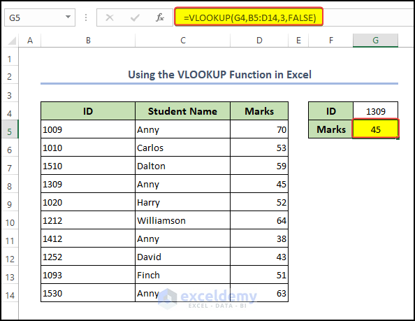
VLOOKUP stands for Vertical Lookup. Now, we will find the marks of Anny by using the VLOOKUP Function.

Syntax: The syntax for the VLOOKUP function is:

=VLOOKUP(lookup_value, table_array, col_index_num, [range_lookup]).

Steps:

• First, we need to enter the following formula in cell G5

Following these steps,  the formula becomes,

• Finally, press Enter on your keyboard.
• After that, you will get your specific data, matched with the ID.

2.2. Use the HLOOKUP Function

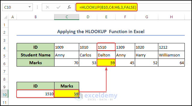
While VLOOKUP searches for matching values in a different column, HLOOKUP searches for matching values within a specific row, hence its name, which stands for Horizontal Lookup. Now, we will find specific data by using the HLOOKUP Function.

Syntax: The syntax for the HLOOKUP function is:

=HLOOKUP(lookup_value, table_array, row_index_num, [range_lookup])
To find specific data while performing the HLOOKUP Function you follow the following instructions,

Steps:

• First, in cell C10 enter the following formula:

• After that, press Enter on your keyboard.
• Finally, after doing these steps you will get your desired marks matched with the ID.

3. Utilize the INDEX-MATCH to Select Specific Data in Excel

Using VLOOKUP has some limitations. The VLOOKUP function can only look up a value from left to right. To avoid this, use the combination of INDEX and MATCH functions instead.
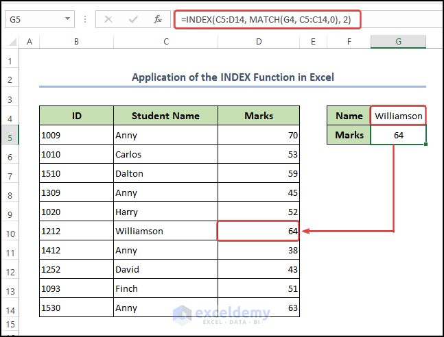
Let’s say, we want to find out the marks of a specific student named Williamson. To find out his marks using INDEX and MATCH functions-
Steps:
● At first, select the cell you want to have the return value in. In our case, we have selected G5
● Then write the below formula in that cell or the formula bar.

Finally, after pressing ENTER on the keyboard, we will get an output value of 64 which is the mark of Williamson.

4. Apply the MATCH Function Only to Return the Position of Specific Data

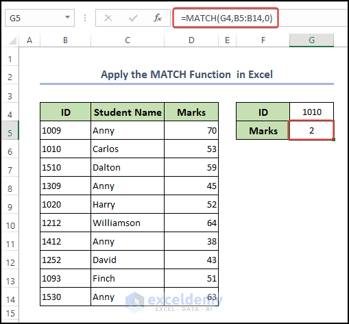
In Excel, the MATCH function investigates a value in an array and returns the relative position of that criterion.

To find a matching value follow the steps:
Steps:
● At first, select cell G6, and enter the following formula:

Here,

• Enter lookup_value like Cell G5 in the parentheses, followed by a comma.
• Then inject the lookup_range, we have B5:B14.
• Now, enter the exact match type 0.
• Then press ENTER on your keyboard button.
• After pressing Enter you can see that the Marks value matched with the ID is now showing in the cell G4.

5. Using the IF Function

While working with Excel you can also select specific data by using the IF function. It is a logical function. In our dataset, we can easily find out if a student passed or failed his/ her examination by using the IF function.

Steps:
Applying the IF function you should follow the steps:

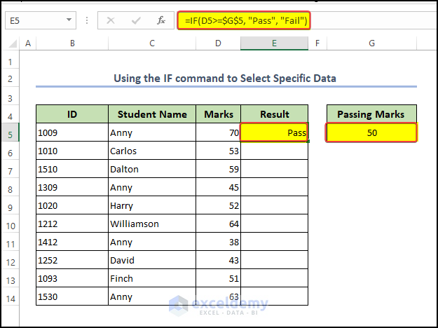
• First, select a cell (i.e, E5), then enter the following formula,

• The main logic in the parentheses is D5>=50
• After that, If D5 is satisfied then he/she will pass. Otherwise, he/she will fail.
• Finally, press the Enter button on your keyboard.

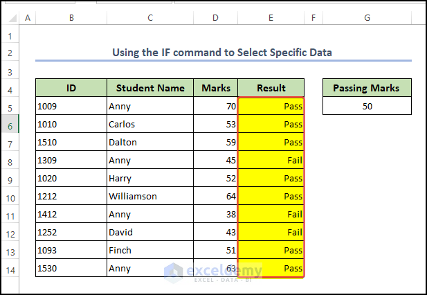
• Then apply the same function to the rest of the cells in the dataset by dragging down the Fill Handle.
• Finally, we got the result of the student by applying the IF function.

Read More: Select a Range of Cells in Excel Formula

Frequently Asked Question

How do I select specific text in Excel?

• Click and drag your mouse cursor over the text you want to select. You should see the text highlight as you drag the cursor.
• If you want to select a larger block of text, you can click and drag the cursor across multiple cells or rows.
• If you want to select non-contiguous cells or text, hold down the “Ctrl” key on your keyboard and click on each cell or section of text you want to select.
• Once you have selected the desired text, you can use any of the standard editing functions in Excel, such as copying, cutting, pasting, formatting, and so on.

How do I isolate specific data in Excel?

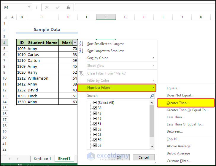
In order to isolate specific data, you can use the Filter tool. Using this you can easily isolate a significant portion of the data of your choice. For example in the image below,

You can apply a filter for a range of cells shown below, and then choose the filter parameter. We applied a filter for the Marks column and then applied a greater-than parameter as shown.

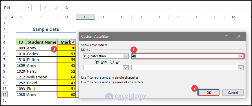
• After clicking on Greater Than there is another window, in that window, enter the value in the parameter box.
• After that, click on
• This will remove any value below 40.

How do I selectively copy text?

You can select specific text using the Filter tool shown above, or you can just use the Ctrl button shortcut. While pressing the Ctrl Button, click on the cell on which you wish to select.Each of those individual cells will then be selected, and you can use them for your own use.

Things to Remember

• Be precise: Make sure you select exactly the data you need, including any headers or labels that are associated with the data. This will help ensure that your calculations and analyses are accurate.
• Consider the type of data: If you are selecting data that includes text, numbers, and formulas, be careful not to accidentally include parts of formulas or formatting that could affect your results.
• Check for hidden data: Excel can sometimes hide data that falls outside the visible range of cells. Make sure you select all relevant data, even if it is hidden.
• Use shortcuts: Excel includes many shortcuts that can make selecting data faster and easier. For example, you can use the “Ctrl” key to select non-adjacent cells, or the “Shift” key to select a range of cells.
• Avoid overwriting data: When copying and pasting data, be careful not to overwrite any existing data that you need to keep. Use a new sheet or a different section of your spreadsheet if necessary.
• Be mindful of cell references: If you are selecting data for use in formulas or functions, make sure you use the correct cell references to ensure that your calculations are accurate.

Download Practice Workbook

Download this practice workbook to exercise while you are reading this article.

Conclusion

In this article, we use multiple Excel features to select specific data in Excel. Here we discussed the Keyboard shortcut, and then used functions like INDEX, HLOOKUP, VLOOKUP, MATCH, IF, etc. Additionally, every single method has its own characteristics and is suitable for the user’s specific needs. That’s why users need to understand which method is going to be best for them and choose accordingly. Hope this article helps to solve your problem.

<< Go Back to Select Range in Excel | Excel Range | Learn Excel