In this Excel tutorial, you will learn how to return multiple values based on single criteria. In the example below we have the list of all the FIFA World Cups that have taken place from 1930 to 2018. We have the Year in Column B, the Host Country in Column C, the Champion countries in Column D, and the Runners-up countries in Column E.
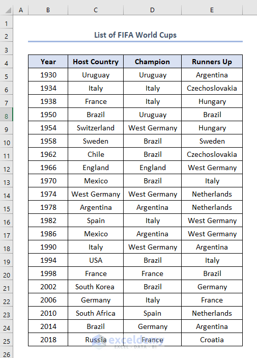
Now we’ll try to extract multiple values based on a single criterion from this data set.
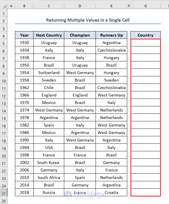
1. Returning Multiple Values Based on a Single Criteria in a Single Cell
First we’ll try to return multiple values in a single cell. We will extract the names of all the champion countries to one column and will add the years in which they became champions to the adjacent cells. Let’s say we want to extract the names of the champion countries in Column G named Country.
- We will use the UNIQUE function of Excel. Enter this formula in cell G5.
=UNIQUE(D5:D25)D5:D25 refers to the Champions.
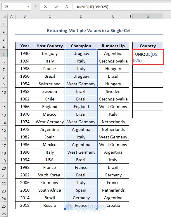
- Press ENTER.
- All the champions are now listed in Column G.
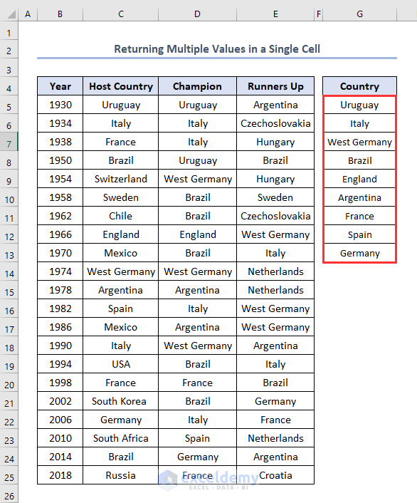
Note: While using Microsoft 365, there is no need to use the Fill Handle to get all the values. All values will appear automatically.
1.1. Using TEXTJOIN and IF Functions
Using a combination of TEXTJOIN and IF functions is a common application to find multiple values based on single criteria. The usage of these two functions mainly finds out the common values of a base value from two or more criteria.
In the following dataset, we have Champion countries in Column G repeated once. We need to find out the Years of these Champion teams in one cell individually.
- To do this, firstly, write the formula in the H5 cell like this.
=TEXTJOIN(",",TRUE,IF($D$5:$D$25=G5,$B$5:$B$25,""))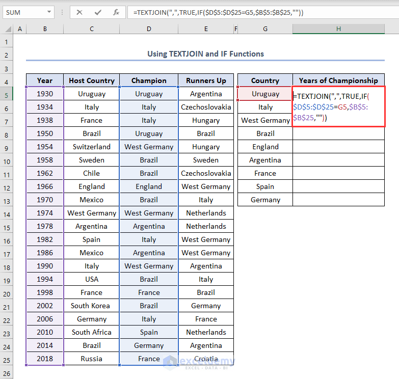
- Secondly, press ENTER to get the output as 1930,1950.
- Thirdly, use the Fill Handle by dragging down the cursor while holding the right-bottom corner of the H5

- Eventually, we’ll get the outputs like this.

Formula Explanation
- Here $B$5:$B$25 is the lookup array. We want to look up for the years. If you want anything else, use that one.
- $D$5:$D$25=G5 is the criteria we want to match. We want to match cell G5 (Uruguay) with the Champion column ($D$5:$D$25). If you want anything else, use that one.
1.2. Combining TEXTJOIN and FILTER Functions
We can also find the same output as the previous one by using the combination of TEXTJOIN and FILTER functions.
- So, firstly, write the formula in the H5 cell like this.
=TEXTJOIN(",",TRUE,FILTER($B$5:$B$25,$D$5:$D$25=G5))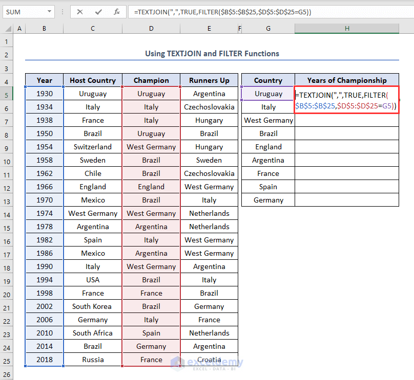
- Secondly, press ENTER.
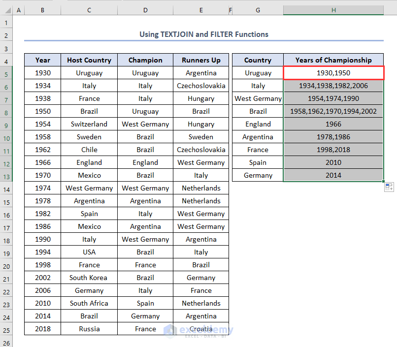
- Thirdly, use the Fill Handle.
- Eventually, we’ll get the output like this.
Formula Explanation
- Here $B$5:$B$25 is the lookup array. We want to look up for the years. If you want anything else, use that one.
- $D$5:$D$25=G5 is the criteria we want to match. We want to match cell G5 (Uruguay) with the Champion column ($D$5:$D$25). If you want anything else, use that one.
2. Return Multiple Values Based on Single Criteria in a Column
The above-mentioned functions are only available in Office 365. Now if you do not have an Office 365 subscription, you can follow these methods and return multiple values based on a criterion in a column.
2.1. Using a Combination of INDEX, SMALL, MATCH, ROW, and ROWS Functions
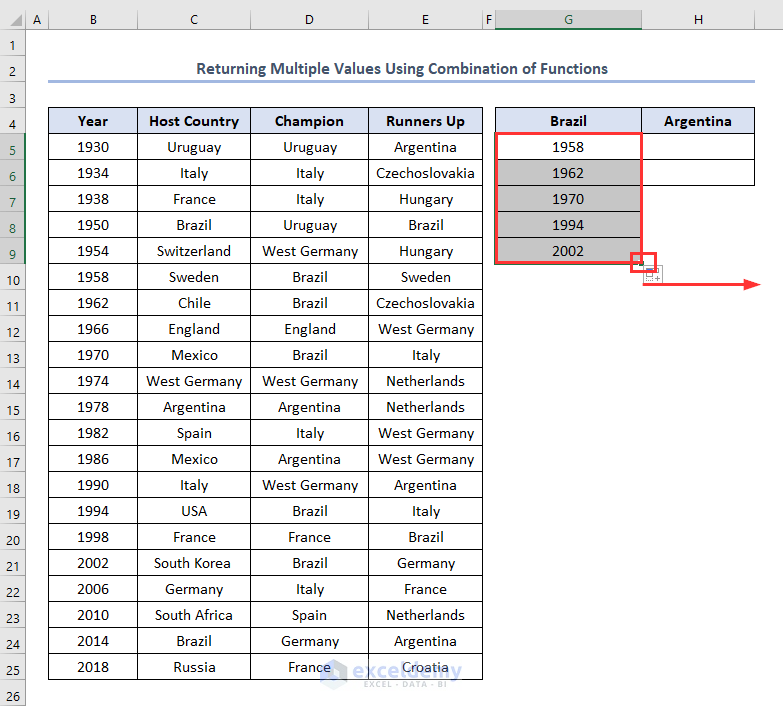
Suppose, we need to find out in which years Brazil became the champion. We can find it by using the combination of INDEX, SMALL, MATCH, ROW, and ROWS functions.
In the following dataset, we need to find it in cell G5.
- So, firstly, write the formula in the G5 cell like this.
=INDEX($B$5:$B$25, SMALL(IF(G$4=$D$5:$D$25, MATCH(ROW($D$5:$D$25),ROW($D$5:$D$25)), ""), ROWS($A$1:A1)))
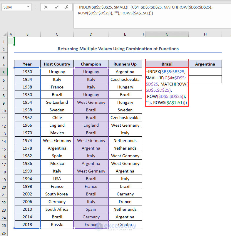
- As this is an array formula, now we need to press CTRL + SHIFT + ENTER.
- Eventually, we’ll find the years in which Brazil became champion as output.
Now, using the above formula you can extract the years of the championship of any other country.
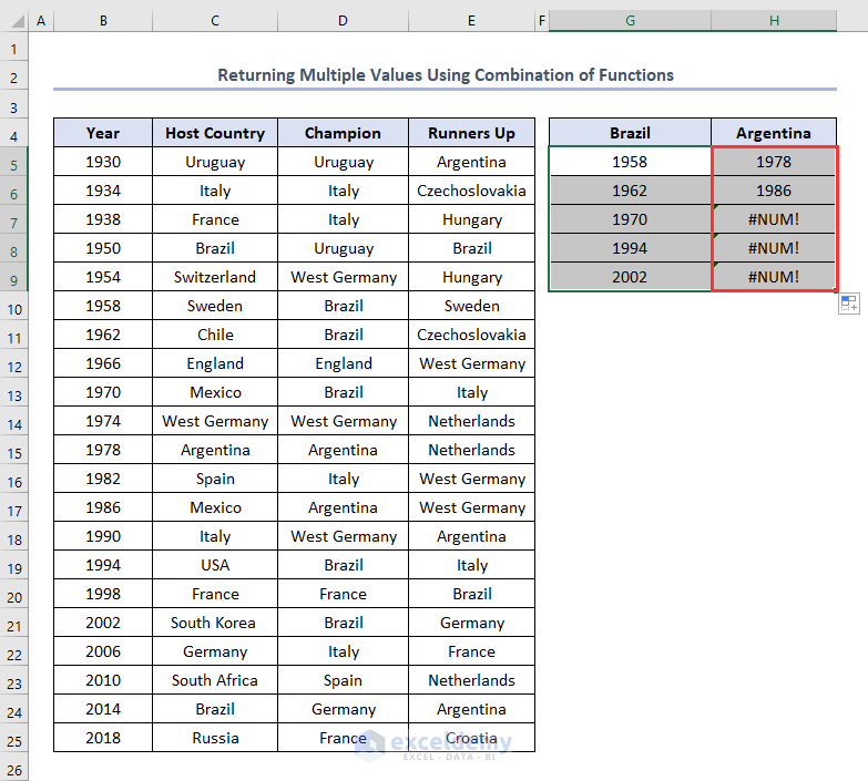
For example, to find out the years when Argentina was champion in Column H, create a new column Argentina adjacent to the one in Brazil, and drag the formula to the right by using the Fill Handle.
Consequently, we’ll find the output like this.
Formula Explanation
- Here $B$5:$B$25 is the lookup array. We look for years. If you have anything else to look up for, use that.
- G$4=$D$5:$D$25 is the matching criteria. We want to match the content of the cell G4, Brazil with the contents of the cells from D5 to D25. You use your criteria.
- Again, $D$5:$D$25 is the matching column. You use your column.
See, we got the years when Argentina was the champion. The years 1978 and 1986.
We can do it for all other countries.
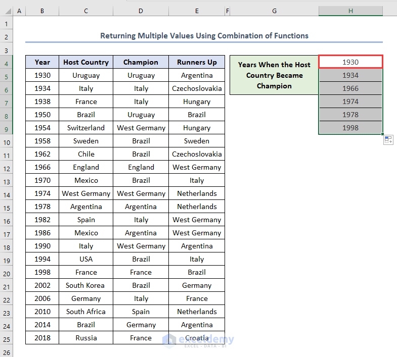
Before moving to the next section, I have one small question for you. Can you find out the years when the World Cup was won by the host countries?
Yes. You have guessed right. The formula will be in the H5 cell like this.
=INDEX($B$5:$B$25, SMALL(IF($C$5:$C$25=$D$5:$D$25, MATCH(ROW($D$5:$D$25),ROW($D$5:$D$25)), ""), ROWS($A$1:A1)))
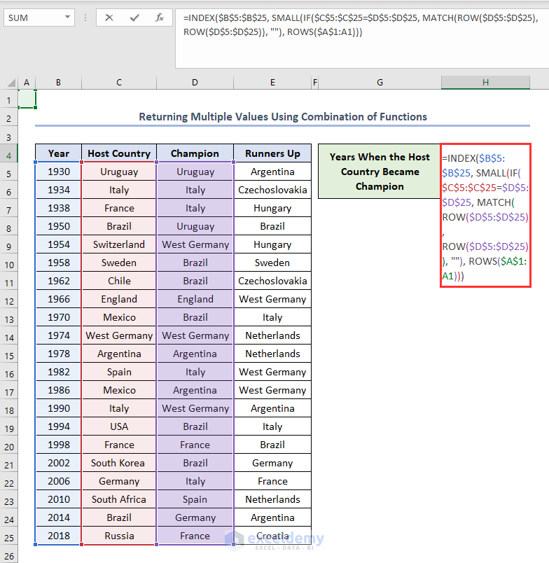
Eventually, the host country became champion in 1930,1934,1966,1974,1978, and 1998.
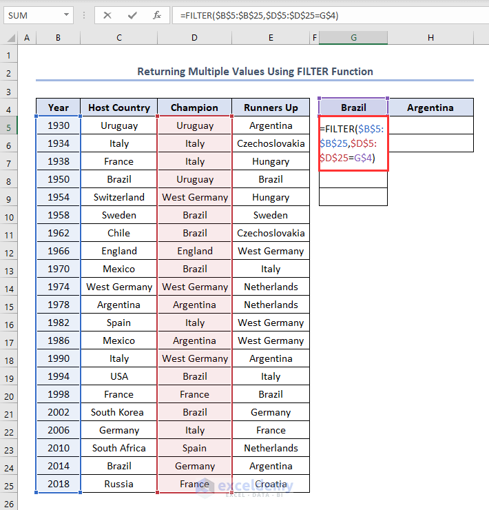
2.2. Applying FILTER Function
If we do not want to use the complex formula mentioned above, we can accomplish the task pretty conveniently using the FILTER function of Excel.
But the only problem is that the FILTER function is available in Office 365 only.
Anyway, the formula in cell G5 to sort out the years when Brazil was the champion will be.
Formula Explanation
- As usual, $B$5:$B$25 is the lookup array. Years in our case. You use your one.
- $D$5:$D$25=G$4 is the matching criteria. You use your one.
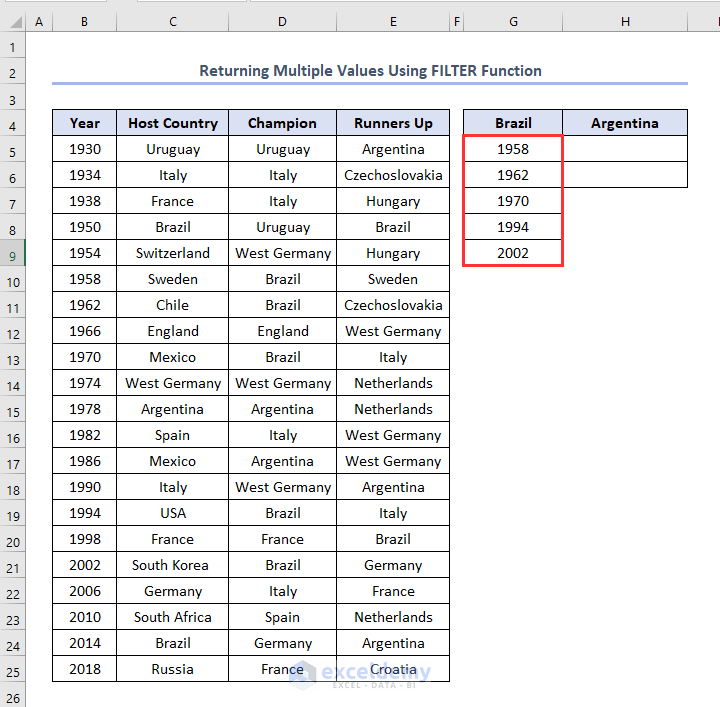
- Secondly, press ENTER to get the outputs like this.
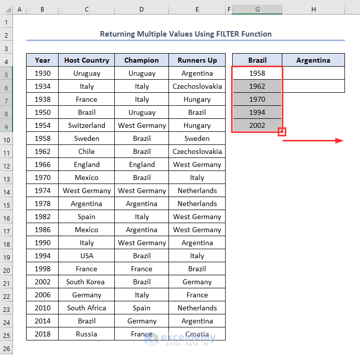
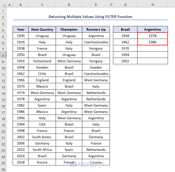
- Now like the earlier method, we can create a new column Argentina just beside Brazil, and drag the Fill Handle to the right to get the Years when Argentina was champion.
Eventually, the output will be like this.
3. Return Multiple Values in Excel Based on Single Criteria in a Row
Finally, if you want, you can return multiple values based on criteria in a row. We can do it by using the combination of IFERROR, INDEX, SMALL, IF, ROW, and COLUMN functions.
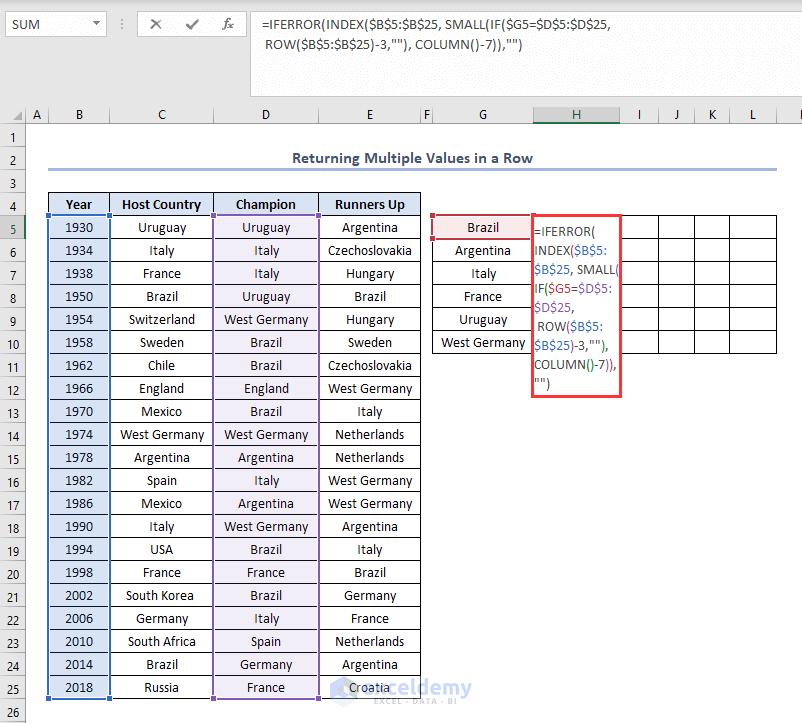
- To find out the years when Brazil was the champion, firstly, select a cell and enter Brazil. In this case, it is G5.
- Secondly, write this array formula in the adjacent cell i.e. H5, and press CTRL + SHIFT + ENTER.
=IFERROR(INDEX($B$5:$B$25, SMALL(IF($G5=$D$5:$D$25,ROW($B$5:$B$25)-3,""), COLUMN()-7)),"")
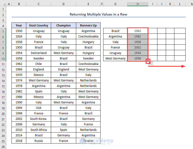
- Thirdly, press ENTER.
- Eventually, we’ll find the years of different specific countries when they became champions first. It will happen automatically in Microsoft 365 without using the Fill Handle.
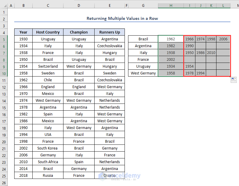
- Now, to find the other years when these countries became champions, just use the Fill Handle
- Consequently, we’ll get the output like this.
Formula Explanation
- Here $B$5:$B$25 is the lookup array. We looked up for years in the range B5 to B25. If you want anything else, use that.
- $G5=$D$5:$D$25 is the matching criteria. I want to match cell G5 (Brazil) with the Champion column (D5 to D25). If you want to do anything else, do that.
- I have used ROW($B$5:$B$25)-3 because this is my lookup array and the first cell of this array starts in row number 4 (B4). For example, if your lookup array is $D$6:$D$25, use ROW($D$6:$D$25)-5.
- In place of COLUMN()-7, use the number of the previous column where you are inserting the formula. For example, if you are inserting the formula in column G, use COLUMN()-6.
Download Practice Workbook
Conclusion
These are the ways to return multiple values based on single criteria in Excel. I have also shown you how to return multiple values based on single criteria in a column and in a row. We have used several Excel functions to do this. I hope you like these data extraction methods.
<< Go Back to Lookup | Formula List | Learn Excel
Get FREE Advanced Excel Exercises with Solutions!

SUPERB VERY GOOD LESSON FORA NOVICE.
THANK YOU SO MUCH
Hello Selam,
You are most welcome.
Regards
ExcelDemy