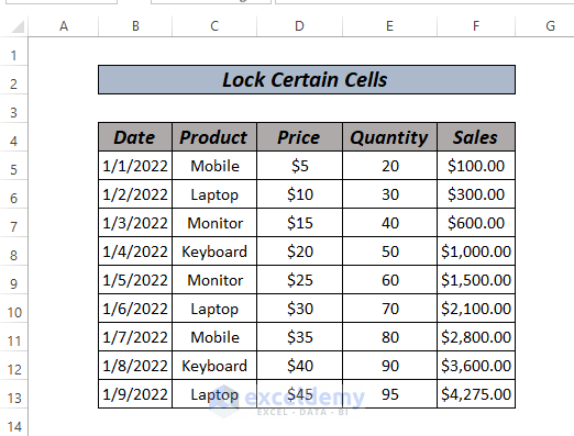
To protect our spreadsheet, we need to know how to lock certain cells in Excel. Locking the whole spreadsheet or certain cells in Excel allows us to protect our data and integrity, and prevent others from deleting formulas and manipulating our data. For your better understanding, we will use a sample dataset containing Date, Product, Price, Quantity, and Sales.
How to Lock Certain Cells in Excel: 4 Simple Ways
In this tutorial, we will see four different methods on how to lock certain cells in Excel. Using our dataset we will show you locking cells containing raw data and formulas.
Method 1: Lock Certain Cells in Excel Using Home Tab
By default, the worksheet is locked. So, first, we need to unlock the entire worksheet then we can lock certain cells as we want.
Steps:
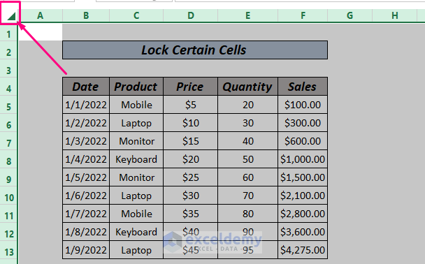
- First, select the entire worksheet by clicking on the sign as shown in the image.
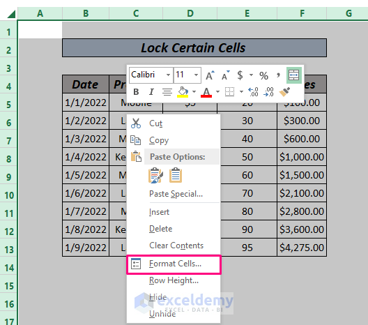
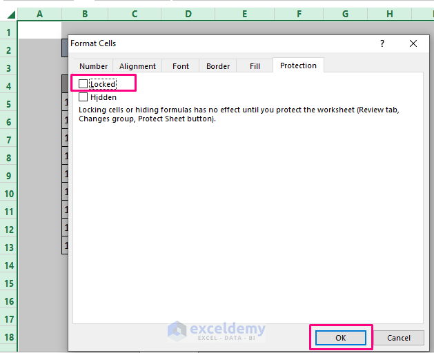
- Now, right-click on the mouse button and select Format Cells.
As we told you earlier, all the cells are by default locked, you can see that.
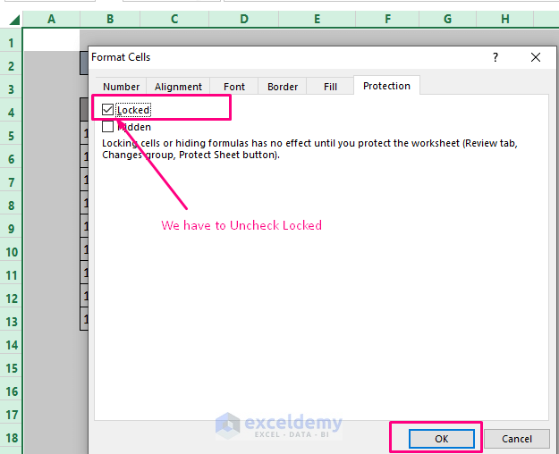
- So, just uncheck the Locked options, and click OK.
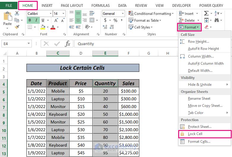
- Now, select the cells we want to lock (here, we want to lock Product and Quantity columns) and go to Home > Format > Lock Cells.
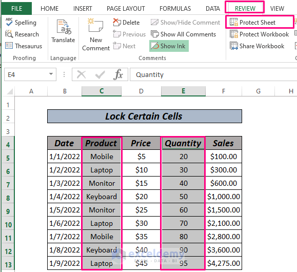
- A dialogue box will pop up. Now, give the password as you like.
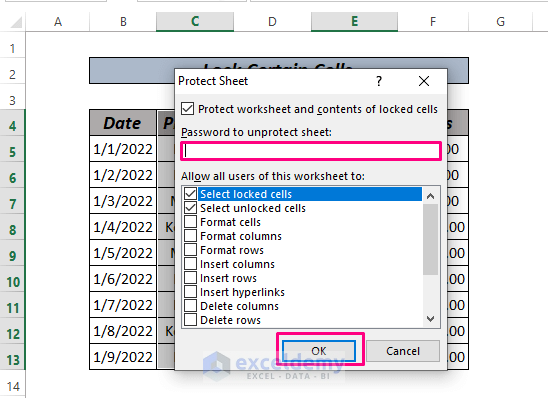
- Clicking OK will ask you to Re-enter the password.
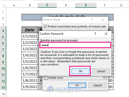
Finally, click OK and done. All the cells from the selected columns will be locked.
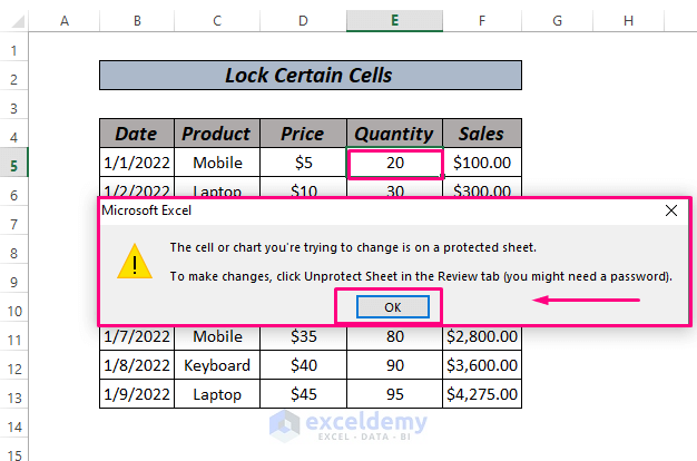
At this point, click on any of the cells in those selected columns and a message box will pop up.
Read More: How to Protect Excel Cells with Formulas
Method 2: Using Format Cells to Lock Certain Cells
Another method to lock certain cells in Excel is the Format Cells option using a shortcut. Here we want to lock all the cells in the Product column.
Steps:
- First, select the entire worksheet by clicking on the sign as shown in the image.
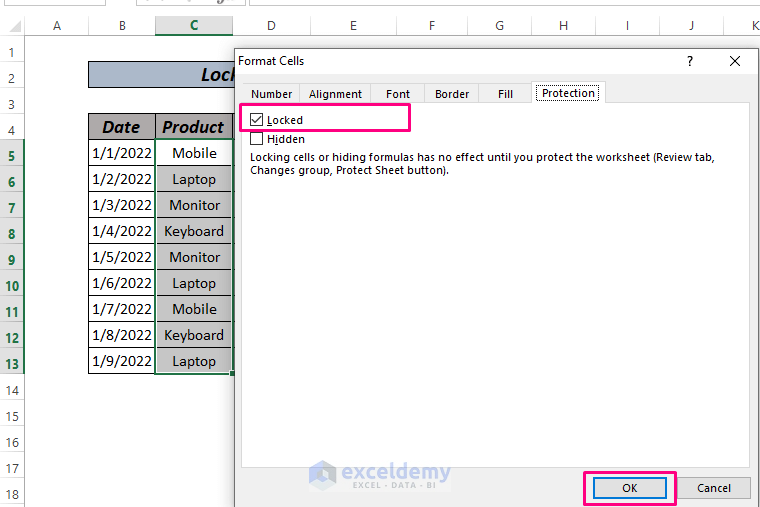
- Now, right-click on the mouse button and select Format Cells.
As we told you earlier, all the cells are by default locked, you can see that.
- So, just uncheck the Locked options and click OK.
- Now, select the cells in Product column and press the CTRL+1 key. This time , check the Locked box, as shown in the image below.
- After that, we have to do all the work from the Review tab. So, from here, we have to follow the methods from Method 1.
Read More: How to Protect Excel Cells with Password
Method 3: Lock Certain Cells Containing Formulas
Till now, we have seen locking certain cells. What if, our dataset is huge and contains formulas. There’s an easy way to lock formula cells in Excel.
Steps:
- First, select the entire worksheet by clicking on the sign as shown in the image.
- Now, right-click on the mouse button and select Format Cells.
As we told you earlier, all the cells are by default locked, you can see that.
- So, just uncheck the Locked options and click OK.
- Now, press CTRL+G and a dialogue box will pop up.
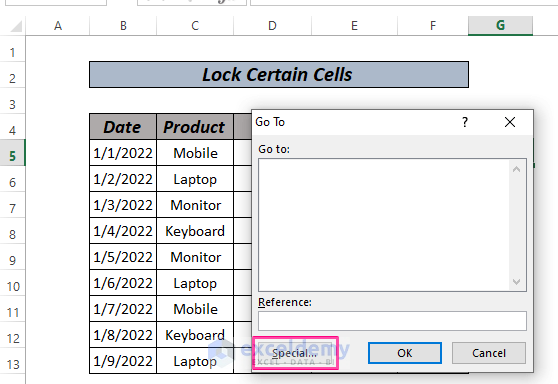
- From, the dialogue box, select Special and another dialogue box will pop up this time. We select the Formulas option from there. Like the image below.
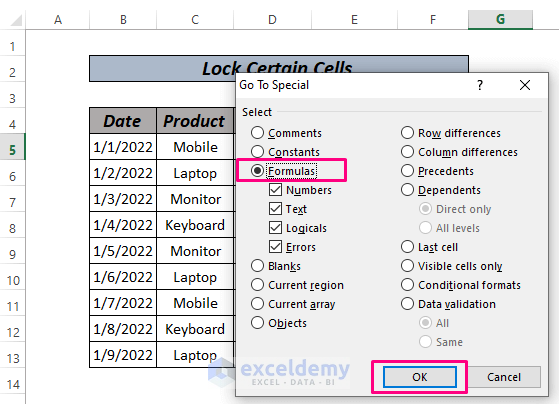
- After clicking OK, all our formula cells will be selected automatically.
From here, all we need to do is, follow either Method 1 or Method 2.
Read More: How to Protect Cells Without Protecting Sheet in Excel
Method 4: VBA to Lock Certain Cells
At the end of this tutorial, we will see a VBA code to lock certain cells in Excel.
Steps:
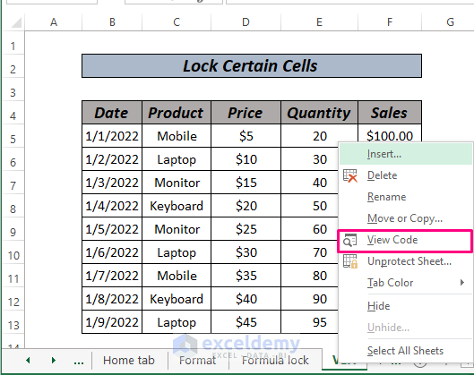
- First, right-click on the sheet and go to View Code.
- After that, copy and paste the VBA code below.
VBA code:
Sub CertainCellLocker()
Cells.Select
Selection.Locked = False
Range("B5:B13,F5:F13").Select
Selection.Locked = True
ActiveSheet.Unprotect Password:="exceldemy"
ActiveSheet.Range("B5:B13,F5:F13").Cells.Locked = True
ActiveSheet.Protect Password:="exceldemy"
End Sub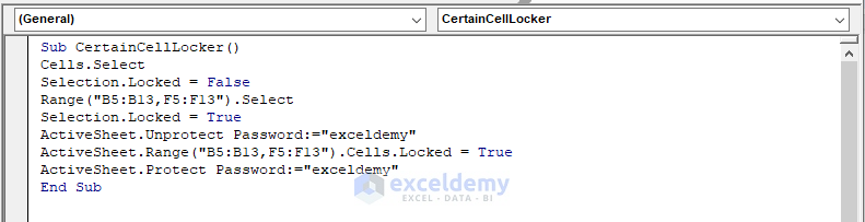
To unlock the by default locked cells, we commanded Selection.Locked = False.
Then, we specified our certain cells by Range(“B5:B13,F5:F13”).Select and locked them through the code Selection.Locked = True.
- After that, press the F5 or play button to run the code.
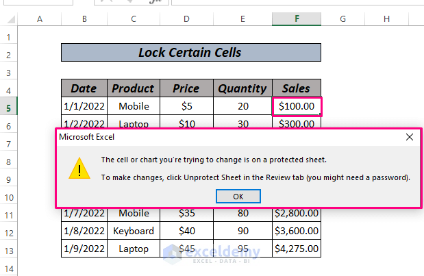
As you can see, from the above image, we locked our desired cells.
Practice Section
The single most crucial aspect in becoming accustomed to these quick approaches is practice. As a result, we’ve attached a practice workbook where you may practice these methods.
Download Practice Workbook
Conclusion
These are 4 different methods on how to lock certain cells in Excel. Based on your preferences, you may choose the best alternative. Please leave them in the comments area if you have any questions or feedback.
Related Articles
- How to Lock Multiple Cells in Excel
- How to Lock a Cell in Excel Formula
- How to Unlock Cells without Password in Excel
- How to Lock Cell Value Once Calculated in Excel
- How to Protect Excel Cells from Deletion
- Protect Excel Cells But Allow Data Entry
- How to Protect Excel Cells from Being Edited
<< Go Back to Protect Excel Cells | Excel Protect | Learn Excel
Get FREE Advanced Excel Exercises with Solutions!

Mahbubur,
Thank you so much for a concise and detailed IFU. I had learned how to do this years ago, but not having done it in a few years left me lost! There are other ways to do it, but to me, this is the “old” way but I still prefer it.
Thanks again.
Hello Lynn,
You are most welcome.
Regards
ExcelDemy