Example with Excel Solver to Minimize Cost

If you are looking for special tricks to know how to minimize cost using Excel solver with example, you’ve come to the right place. This article will discuss the details of all the examples of minimizing cost. Let’s follow the complete guide to learn all of this.

What Is Solver in Excel?

Solver is a Microsoft Excel add-in program. The Solver is part of the What-If Analysis tools that we can use in Excel to test different scenarios. We can solve decision-making issues using the Excel tool Solver by finding the most perfect solutions. They also analyze how each possibility impacts the worksheet’s output.

How to Add Solver to Excel

You can access Solver by choosing Data ➪ Analyze ➪ Solver. Sometimes it may happen that this command isn’t available, you have to install the Solver add-in using the following steps:

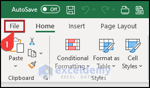
First of all, choose the File tab.

Secondly, select Options from the menu.

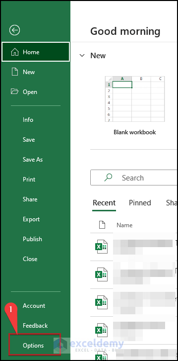
Thus, the Excel Options dialog box appears.
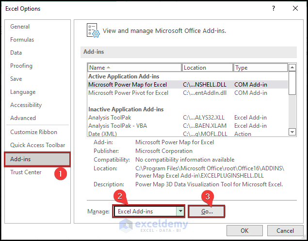
Here, go to the Add-Ins tab.
At the bottom of the Excel Options dialog box, select Excel Add-Ins from the Manage drop-down list and then click Go.

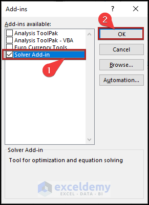
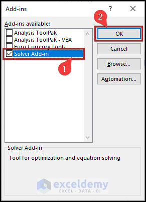
Immediately, the Add-ins dialog box appears.
Then, place a checkmark next to Solver Add-In, and then click OK.

Another way: Also, we can install the Solver add-in using the Developer tab. Just follow along.
Initially, proceed to the Developer tab.
Secondarily, click on Excel Add-ins on the Add-ins group.

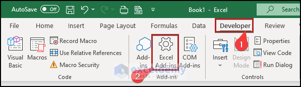
Again, it opens the Add-ins wizard.
After that, do the similar tasks that we’ve done above.

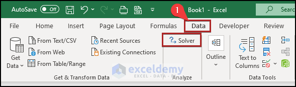
Once you activate the add-ins in your Excel workbook, they will be visible on the ribbon.
Just move to the Data tab.
And, you can find the Solver add-ins on the Analyze group.

How to Use Solver in Excel

Before going into more detail, here’s the basic procedure for using Solver:

First of all, set up the worksheet with values and formulas. Make sure that you have formatted cells correctly; for example, the maximum time you can’t produce partial units of your products, so format those cells to contain numbers with no decimal values.
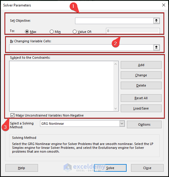
Next, choose Data ➪ Analysis ➪ Solver. The Solver Parameters dialog box will appear.
Afterward, specify the target cell. The target cell also is known as the objective.
Then, specify the range that contains the changing cells.
Specify the constraints.
If necessary, change the Solver options.
Let the Solver solve the problem.

Introduction to Solver Parameters

The Excel Solver determines the best solution based on the objective cell formula.

Firstly, let’s get introduced to the nomenclatures used in the Solver Parameters dialog box. While using the solver, that’ll be beneficial. These are the definitions for the terms:

Objective Cell: It is simply a single cell with something like a formula in it. The constraint cells’ limitations are applied to the decision-based formula in the cell. The objective cell’s value can be decreased, increased, or fixed at the provided threshold.

Variable Cells: Variable cells are made up of variable data that the Solver modifies to accomplish the goal.

Constraint Cells: These are the constraints that the solution to the situation at hand must adhere to. On the other hand, these are the prerequisites that must be met.

Example with Excel Solver to Minimize Cost: 2 Suitable Examples

In the following section, we will use two effective and tricky examples of the Excel solver to minimize cost. This section provides extensive details on these examples. In the first example, we’re going to find alternative options for shipping materials keeping total shipping costs at a minimum level. Say a company has warehouses in St. Louis, Los Angeles, and Boston. Six retail outlets are situated all over the United States. These retail outlets take orders from customers. The company then ships products from one of the warehouses. The company’s target is to meet the product needs of all six retail outlets from available inventory in the warehouses. While shipping products to outlets, the company wants to keep shipping charges as low as possible.

You should learn and apply these to improve your thinking capability and Excel knowledge. We use the Microsoft Office 365 version here, but you can utilize any other version according to your preference.

1. Minimize Shipping Cost

Here, we will demonstrate how to minimize shipping costs in Excel. This is the first example of minimizing cost using Excel solver. We will use SUM and SUMPRODUCT functions for calculating different parameters. Our Excel dataset will be introduced to give you a better idea of what we’re trying to accomplish in this article.

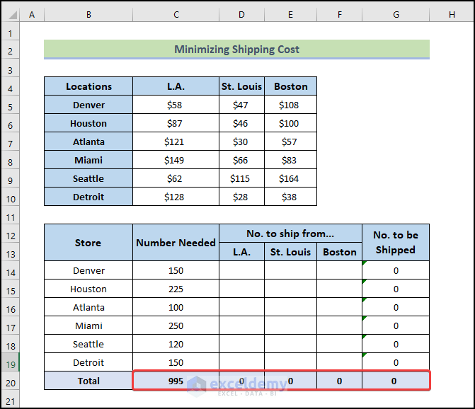
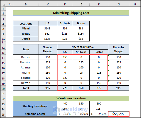
Shipping Costs Table: This table contains the cell range B4:E10. This is a matrix that holds per-unit shipping costs from each warehouse to each retail outlet. For example, the cost to ship a unit of a product from Boston to Detroit is $38.

Product needs of each retail store: This information appears in the cell range C14:C19. For example, the retail outlet in Houston needs 225, Denver needs 150 units, Atlanta needs 100 units, and so on. C18 is a formula cell that calculates the total units needed from the outlets.

No. to ship from: Cell range D14:F19 holds the adjustable cells. These cell values will be varied by Solver. We have initialized these cells with a value of 25 to give Solver a starting value. Column G contains formulas. This column contains the sum of units the company needs to ship to each retail outlet from the warehouses. For example, G14 shows a value of 75. The company has to send 75 units of products to the Denver outlet from three warehouses.

Warehouse inventory: Row 21 contains the amount of inventory at each warehouse. For example, the Los Angeles warehouse has 400 units of inventory. Row 22 contains formulas that show the remaining inventory after shipping. For example, Los Angeles has shipped 150 (see, row 18) units of products, so it has the remaining 250 (400-150) units of inventory.

Calculated shipping costs: Row 24 contains formulas that calculate the shipping costs.

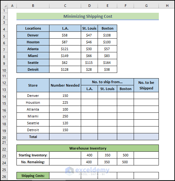
The solver will fill in the values in the cell range D14:F19 in such a way that will minimize the shipping costs from the warehouses to the outlets. In other words, the solution will minimize the value in cell G24 by adjusting the values of cell range D14:F19 fulfilling the following constraints:

The number of units demanded by each retail outlet must equal the number shipped. In other words, all the orders will be filled. The following specifications can express these constraints:

C14=G14, C16=G16, C18=G18, C15=G15, C17=G17, and C19=G19

The number of units remaining in each warehouse’s inventory must not be negative. In other words, a warehouse can’t ship more than its inventory. The following constraint shows this: D24>=0, E24>=0, F24>=0.
The adjustable cells can’t be negative because shipping a negative number of units makes no sense. The Solve Parameters dialog box has a handy option: Make Unconstrained Variables Non-Negative. Make sure this setting is enabled.
Let’s walk through the following steps to do the task.

📌 Steps:

First of all, we will be setting some necessary formulas. To calculate No. to be shipped, type the following formula.

=SUM(D14:F14)

Then, press Enter.

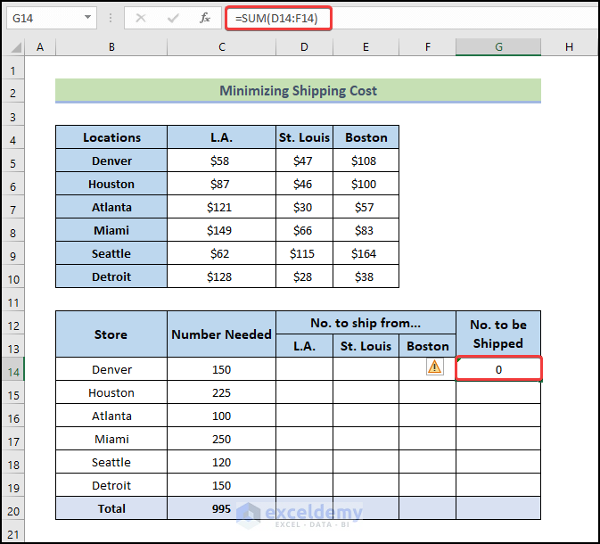
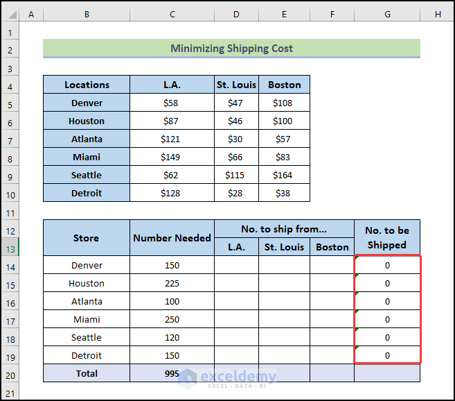
Next, drag the Fill Handle icon up to cell G19 to fill the other cells with the formula.
Therefore, the output will look like this.

Afterward, to calculate the total, type the following formula.

=SUM(C14:C19)

Then, press Enter.

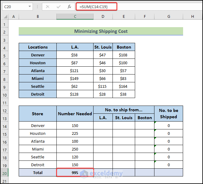
Next, drag the Fill Handle icon to the right up to cell G20 to fill the other cells with the formula.
Therefore, the output will look like this.

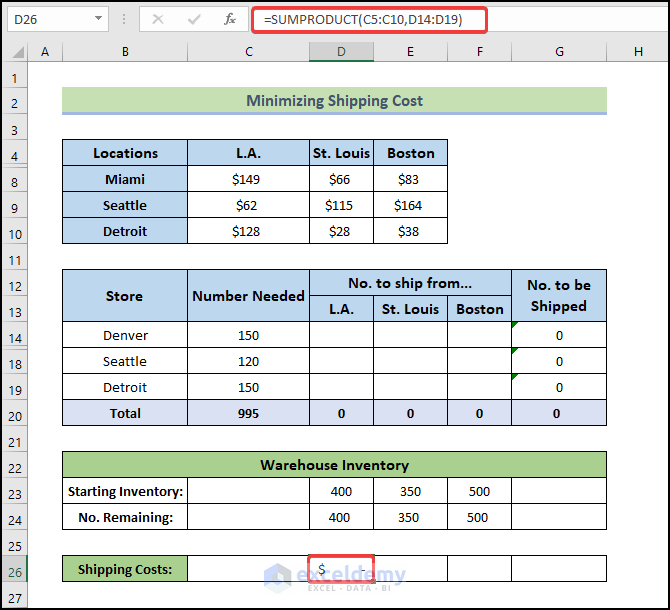
Afterward, to calculate the shipping costs, type the following formula.

=SUMPRODUCT(C5:C10,D14:D19)

Then, press Enter.

Next, drag the Fill Handle icon to the right up to cell F26 to fill the other cells with the formula.
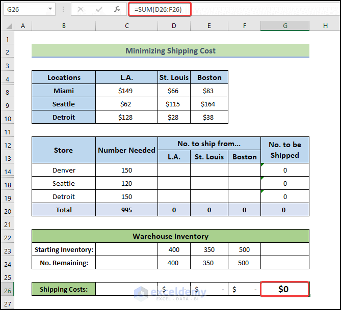
Next, type the following formula in cell G26.

=SUM(D26:F26)

Then, press Enter.
Therefore, the output will look like this.

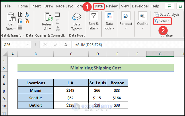
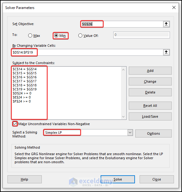
To open the Solver Add-in, go to the Data tab and click on Solver.

Next, fill the Set Objective field with this value: $G$26.
Then, select the radio button of the Min option.
Select cell $D$14 to $F$19 to fill the field By Changing Variable Cells. This field will show then $D$14:$F$19.
Now, Add constraints one by one. The constraints are: C14=G14, C16=G16, C18=G18, C15=G15, C17=G17, C19=G19, D24>=0, E24>=0, and F24>=0. These constraints will be shown in the Subject to the Constraints field.
Afterward, select the Make Unconstrained Variables Non-Negative check box.
Finally, select Simplex LP from the Select a Solving Method drop-down list.

Now, click on the Solve button. The following figure shows the Solver Results dialog box. Once you click OK, your result will be displayed.

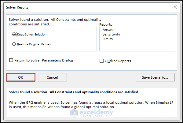
The Solver displays the solution shown in the following figure.

2. Minimize Production Cost

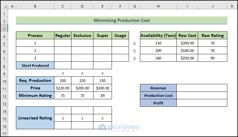
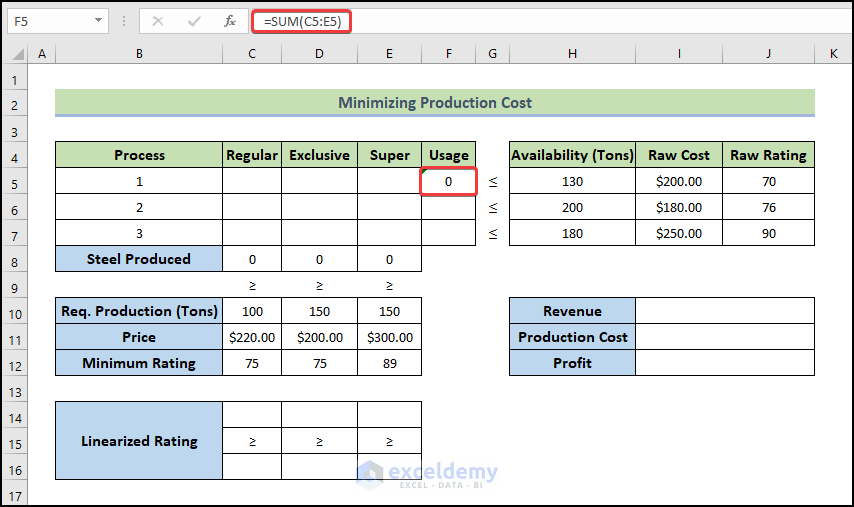
This is the second example to minimize cost using Excel solver. With the following dataset, we will mix different raw materials to produce different types of steel, such as regular, exclusive, and super-quality steel. There is data about the availability and cost of these raw materials, as well as their quality rating. Additionally, we established the required amount of production, the price per ton of different classes of steel, and their minimum rating. We also have a parameter called the Linearized Rating. We will use SUM and SUMPRODUCT functions for calculating different parameters.

Let’s walk through the following steps to minimize production costs using an Excel solver.

📌 Steps:

First of all, we will be setting some necessary formulas. Type the following formula in cell F5.

=SUM(C5:E5)

The formula uses the SUM function to calculate the total amount of the type 1 Steel (Regular, Exclusive, and Super) that will be produced from the first available resources.

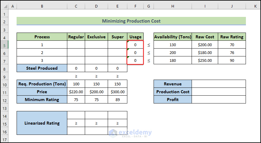
Then, press Enter.

Next, drag the Fill Handle icon up to cell F7 to fill the other cells with the formula.
Therefore, the output will look like this.

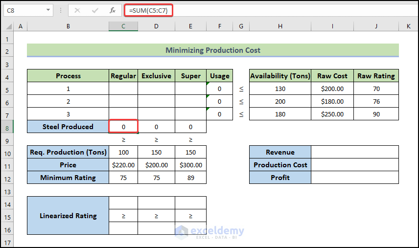
Later, type the following formula for the calculation of the total Regular Steel production amount.

=SUM(C5:C7)

Then, press Enter.
Next, drag the Fill Handle icon up to cell E8 to fill the other cells with the formula.
Therefore, the output will look like this.

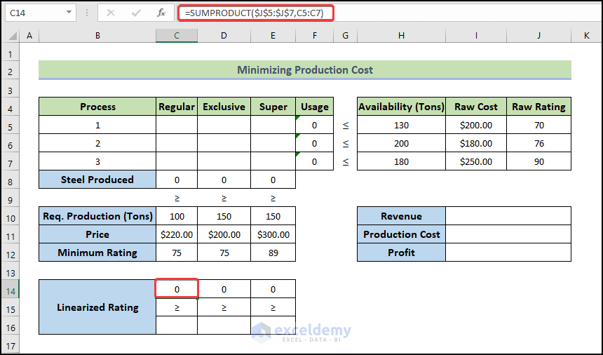
Similarly, write down the formula below in cell C14 to calculate the Linearized Rating and fill the adjacent cells up to E14.

=SUMPRODUCT($J$5:$J$7,C5:C7)

Then, press Enter.
Therefore, the output will look like this.

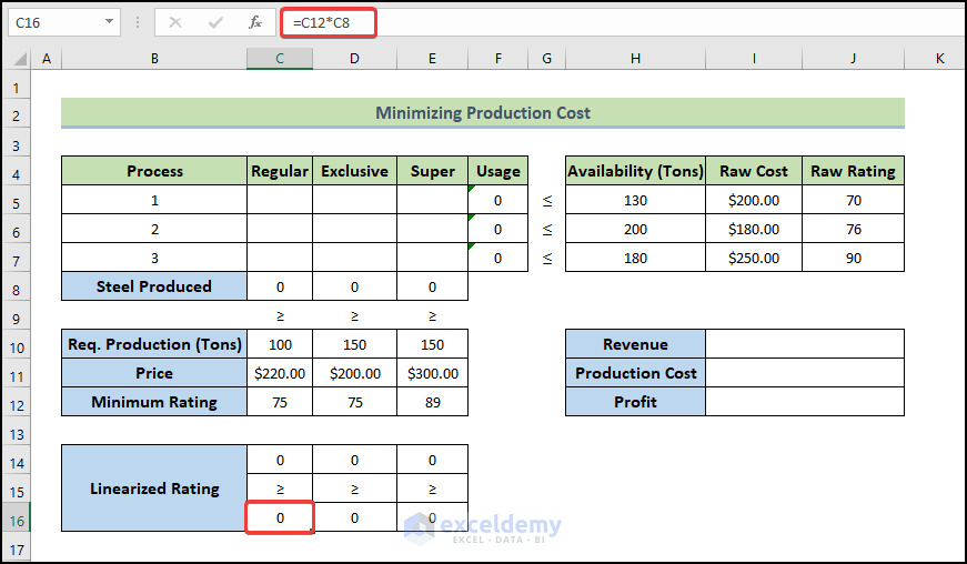
After that, type the following formula C16, and fill the cells up to E16.

=C12*C8

Then, press Enter.
Therefore, the output will look like this.

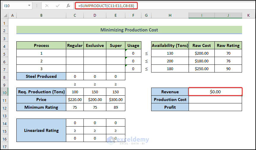
Next, write down the formula below in cell I10 to determine the Revenue.

=SUMPRODUCT(C11:E11,C8:E8)

Then, press Enter.
Therefore, the output will look like this.

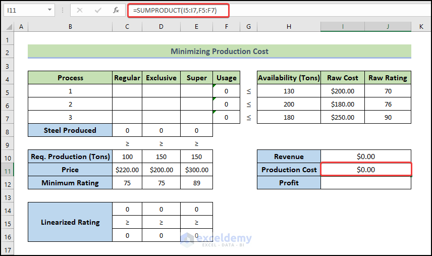
To calculate the production cost, use the following formula.

=SUMPRODUCT(I5:I7,F5:F7)

Then, press Enter.
Therefore, the output will look like this.

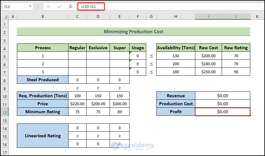
The following formula will return the Profit.

=I10-I11

Then, press Enter.
Therefore, the output will look like this.

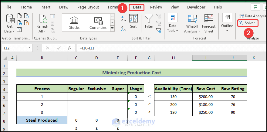
To open the Solver Add-in, go to the Data tab and click on Solver.

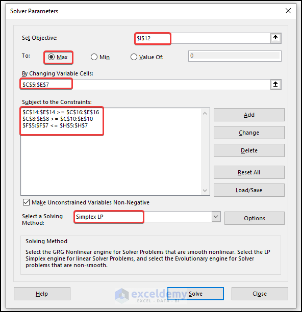
After that, to enter the Subject, Changing Variable, and Constraints, please follow the link of Method 1 that will lead you to the process. I’ll simply explain these inequalities in the following description.
We want to maximize the profit amount, so we reference the cell that contains profit (I12).
Next, our changing variables are the Steel products, so this range will be C5:E7 where the amount of production will be stored.
After that, we added some constraints. The Linearized Raw Rating will be greater than or equal to the Linearized Minimum Required Rating, so the range C14:E14 will be greater or equal to C16:E16.
Thereafter, the production amount will be greater than the required amount. So the range C8:E8 will be greater than C10:E10.
And the usage of raw materials will be lower than the available raw materials. So the range F5:F7 will be greater than H5:H7.

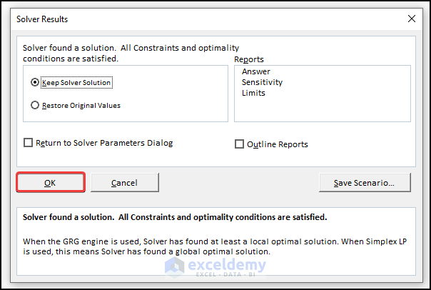
After clicking on Solve, you will get the following window. Next, click on OK.

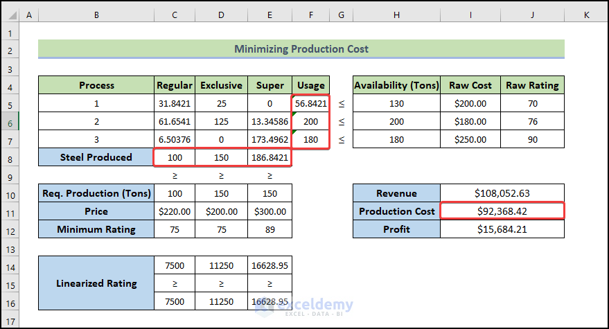
Therefore, you will get the values of how much Raw Materials you should use to get the minimum production cost.
In addition, you will also get the results of Revenue, Cost of production, and Profit.

Download Practice Workbook

Download this practice workbook to exercise while you are reading this article. It contains all the datasets in different spreadsheets for a clear understanding. Try it yourself while you go through the step-by-step process.

Minimize Cost.xlsx

Conclusion

That’s the end of today’s session. I strongly believe that from now on, you may learn how to minimize cost using Excel Solver with example. If you have any queries or recommendations, please share them in the comments section below. Keep learning new methods and keep growing!

<< Go Back to Excel Solver Examples | Solver in Excel | Learn Excel

Get FREE Advanced Excel Exercises with Solutions!

4 Comments

[email protected] Sep 15, 2016 at 9:09 AM

Cannot download example file. It keeps directing me to mailchimp and then I’m seeing error because I’m already subscribed.
- Reply
  Kawser Sep 15, 2016 at 11:21 AM
  
  Check your email please, Smith!
Ahmed Mar 4, 2021 at 8:26 AM

Hi,
I hope you can help me in that using excel

The Kellogg’s Cornflake Company began in 1906 with the Kellogg brothers who originally ran a sanatorium in Michigan, USA. They experimented with different ways to cook cereals without losing the goodness. Their philosophy was ‘improved diet leads to improved health’. Between 1938 and the present day Kellogg’s opened manufacturing plants in the UK, Canada, Australia, Latin America and Asia. Kellogg’s is now the world’s leading breakfast cereal manufacturer. Its products are manufactured in 3 countries; Belgium (location 50,4) with total capacity 25000 tons and distribution costs per unit 6$; China (location 39, 116) with total capacity 28000 tons and distribution costs per unit 9$; and France (location 48, 2) with total capacity 37000 tons and distribution costs per unit 5$, while sold in more than 3 countries; Greece (location 37, 23) with total demand 15000 tons and distribution costs per unit 9$; Ireland (location 53, 6) with total demand 18000 tons and distribution costs per unit 4$; and Luxembourg (location 49, 6) with total demand 28000 tons and distribution costs per unit 9$. It produces a wide range of cereal products, including the well-known brands of Kellogg’s Corn Flakes, Rice Krispies, Special K, Fruit n’ Fibre, as well as the Nutri-Grain cereal bars. Kellogg’s business strategy is clear and focused: • to grow the cereal business – there are now 40 different cereals • to expand the snack business – by diversifying into convenience foods • to engage in specific growth opportunities.

Questions
1. In order to minimize total distribution costs, design a facility location model to determine the right location of establishing a distribution center.
2. Design a distribution network and generate an answer report to determine the flow of goods between suppliers and markets.
3. Is it feasible to shut down one supply markets to minimize total costs if you know that the fixed costs are as follows: Belgium (18000 $), China (17000 $), and France (19000$)? Generate an answer report to shows your results.
- Reply
  Kawser Mar 5, 2021 at 10:47 PM
  
  Hi Ahmed,
  I am keeping a note of your problem, hope we shall be able to make a solution to this.
  Thanks.