In this article, we will show you two quick methods for how to use the INDEX and MATCH functions for multiple criteria without an array in Excel. Two of the most widely used functions of Excel are the INDEX function and the MATCH function, which can be used to match multiple criteria using both array formula and without array formula. Today we are going to show you how you can sort out some data matching multiple criteria in Excel using a non-array formula.
INDEX Function
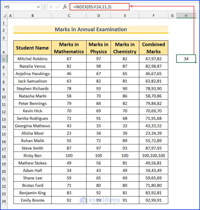
Let us look at the data set again. Assume that someone asked you how much the 11th student obtained in physics. How will you find that? If you do not have any idea about the INDEX function, you will probably count 1… 2… 3.. in the Student Name column, starting from Mitchel Robbins, up to 11. Then you will see what the mark of that student in number 11 in Physics is. In this case, it is Alisha Moor. She achieved a 34 in physics. But you can find this out quite comfortably using Excel’s INDEX Function.
The INDEX function takes three arguments.
- A range of cells from which you want to sort out the datum. In our case it is B5:E24. From the name of the first student, Mitchel Robbins to the number obtained in Chemistry by the last student Emily Bronte, 91.
- The number of the row of the datum which you want to find out, within the range of cells. As here we want to know about the 11th student, the row number here is 11.
- Also the number of the column of the datum which you want to find out, within the range of cells. As here we want to know about the marks in Physics, the column number here is 3.
- So, the syntax for the INDEX Function is:
=INDEX(range,row_number,column_number)
- And in this case, the formula will be:
=INDEX(B5:F24,11,3)
If you select any cell and insert this formula there, you will get the datum of row number 11 and column number 3, from the range of cells B5:E24. In our case, it is 34 points achieved by the 11th student, Alisha Moor.
Points to Keep in Mind
- If you have only one row in the range, inserting the row number is optional. Excel will automatically take it as 1.
- Again If you have only one column in the range, inserting the column number is optional. Excel will automatically take it as 1.
- If you enter any row number or column number that falls out of the range, Excel will raise a reference error (#REF!).
- Also If you enter 0 in place of the row number, Excel will return the whole column as output. But that will work like an array formula then.
- So you have to select multiple (the required number of) cells and press Ctrl+Shift +Enter.
- And If you enter 0 in place of the column number, Excel will return the whole row as output. But that will work like an array formula too.
- So you have to select multiple (the required number of) cells and press Ctrl+Shift +Enter.
This is the array form of the INDEX function. Besides this, there is another form of the INDEX function, called the reference form. That is not necessary here.
MATCH Function
Now, let us discuss the MATCH function of Excel. The syntax of the MATCH function is:
=MATCH(lookup_value, lookup_array, match_type)
The MATCH function takes 3 arguments.
- A specific text or number.
- A range of cells.
- Match type (-1, 0, 1). 0 for an exact match.
Then it returns the position of the cell within the range that is matched with the specific text or number. Going back to our dataset, if we select any cell and enter the formula
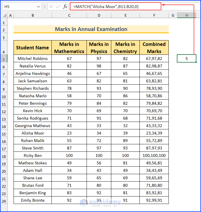
=MATCH("Alisha Moor",B11:B20,0)
It will return 5 because Alisha Moor is in the 5th position in the range from B11 to B20.
Points to Keep in Mind:
- If the MATCH function does not get any match, it returns a Value not Available (#N/A!) error.
- The MATCH function does not distinguish between uppercase and lowercase letters.
Use INDEX MATCH for Multiple Criteria Without Array: 2 Handy Approaches
We will show you two quick methods to achieve our goal. Now, let’s go back to our main point. How to sort out the student obtaining a 100 in all three subjects? There are 3 criteria here.
- 100 in Mathematics, which is column B.
- Also, 100 in Physics, is column C.
- And 100 in Chemistry, that is column D.
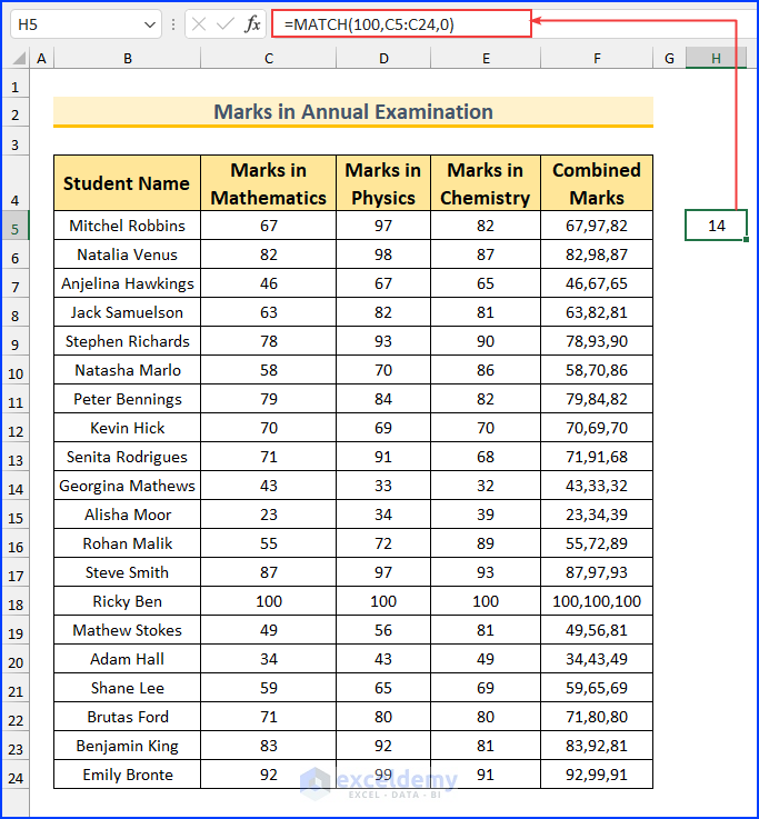
Let’s try for one criterion first. Sort out the student with marks 100 only in mathematics. First, we get the position of the cell in column C, which contains 100 in the range C5 to C24. We shall use the MATCH function here. The formula will be:
=MATCH(100,C5:C24,0)
And you will get 14 because in the 14th cell of column C, there is a 100.
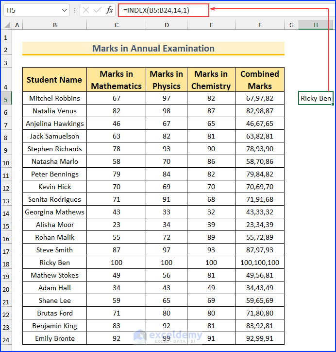
Now use this value to find out the name of the student. It is pretty straightforward. Use the INDEX function to sort out the 14th value in the Student Name column, in the range B5 to B24.
So the formula will be
=INDEX(B5:B24,14,1)
And you will get Ricky Ben.
So the total formula will be
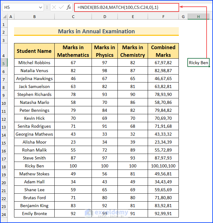
=INDEX(B5:B24,MATCH(100,C5:C24,0),1)
Use this and you will get the same result, Ricky Ben.
Now we sorted out the data with one criterion. But how can we do this for multiple criteria without using an array formula? Here we are showing two ways.
Method 1: Using Helper Column
This is the easier one. First, merge the columns to which your criteria belong into a new column. Here, the three criteria are 100 in mathematics, 100 in physics, and 100 in chemistry. They belong to columns C, D, and E, respectively. So, we combine them into a new column, F, using the CONCATENATE function.
Steps:
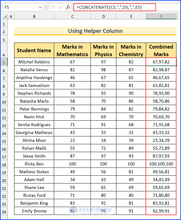
- To merge them, you can either use this formula in the first cell of column F, F5.
=CONCATENATE(C5,",",D5,",",E5)
- Then, drag the Fill Handle to AutoFill the formula into the rest of the cells.
- Or you can directly merge them into F5 by using the ampersand symbol (&) and then, drag the Fill Handle.
=C5&","&D5&","&E5
- In both cases, you will find the numbers of three subjects of each student merged into one column F like this.
- Then consider this as a single criterion and use the INDEX and MATCH formula for a single criterion, shown earlier. In this case, the formula will be –
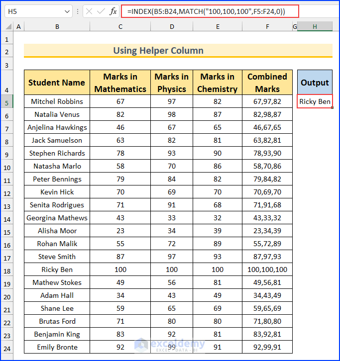
=INDEX(B5:B24,MATCH("100,100,100",F5:F24,0))
- And you will get Ricky Ben because he is the one with 100 in all three subjects.
Special Note: Within the MATCH function, in the first argument (lookup_value), we covered that between apostrophes (“”). Though they were numbers before being merged, after being merged they were converted to text. That’s why we had to use apostrophes (“”).
Method 2: Applying Nested INDEX and MATCH Functions
In this section, we’ll demonstrate how to use nested INDEX and MATCH functions to match multiple criteria at once. This is a bit complex to understand. However, we are showing you step by step so that you can understand clearly.
Steps:
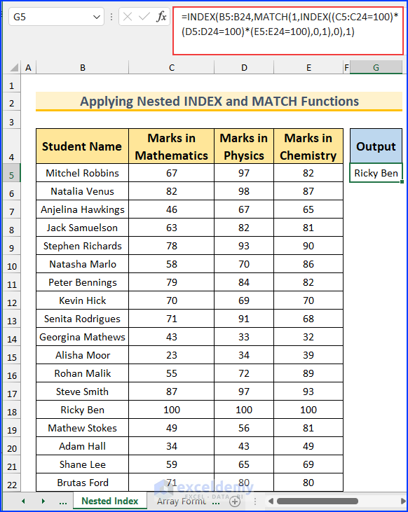
- To begin with, type the following formula in cell G5 and press Enter.
=INDEX(B5:B24,MATCH(1,INDEX((C5:C24=100)*(D5:D24=100)*(E5:E24=100),0,1),0),1)
Formula Breakdown
- C5:C24=100
- Firstly, we are comparing 100 with each mark in Mathematics with this part of the formula. It will return an array of Boolean values, True or False. True if any mark is equal to 100, and False otherwise.
- Secondly, we are doing the same for marks in Physics and Chemistry.
- (C5:C24=100)*(D5:D24=100)*(E5:E24=100)
- Thirdly, we multiply the three values from the previous steps. Despite having Boolean values, they will be converted to numbers, 1 and 0, after multiplication. As anything multiplied by 0 is 0, after multiplication, the resultant array will contain 1 only if there was 1 in all the cells of the row before multiplication.
- In other words, in the resultant array, only the position where marks in all 3 subjects are 100, will have a 1. All others will have 0.
- INDEX((C5:C24=100)*(D5:D24=100)*(E5:E24=100),0,1)
- Then, we enter this resultant array within an INDEX function as range, while keep row number is 0, and column number to 1.
- As the row number is 0, the INDEX function will return the column with the number 1, which means the resultant array which we used as the range.
- MATCH(1,INDEX((C5:C24=100)*(D5:D24=100)*(E5:E24=100),0,1),0)
- Afterward, we enter this into a MATCH function and find out if there is any 1 within it.
- INDEX(B5:B24,MATCH(1,INDEX((C5:C24=100)*(D5:D24=100)*(E5:E24=100),0,1),0),1)
- Finally, we enter it within another INDEX function as the row number, with the name of the students as its range and the column number as 1.
- It will return the Name of the Student in that position. And we will get the student with 100 in all three subjects. In our case, that is Ricky Ben.
- So, we can sort out any data from any data set using this formula, maintaining multiple criteria. The best thing is that it is a non-array formula. That means you do not need to press Ctrl+Shift+Enter to enter this formula. Only pressing Enter will do.
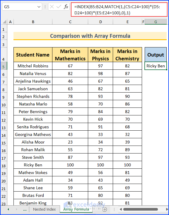
Comparison with Array Formula
There is a comparatively shorter formula for using INDEX MATCH for multiple criteria without an array. But this is an array formula. After writing this into the formula bar, you have to press Ctrl+Shift+Enter to enter this. Excel will automatically put curly braces ({}) around this in the formula bar, as a sign of an array formula. However, we are using the Microsoft 365 version, so we can simply press Enter and it will not show a curly bracket for this version. The the formula is –
=INDEX(B5:B24,MATCH(1,(C5:C24=100)*(D5:D24=100)*(E5:E24=100),0),1)
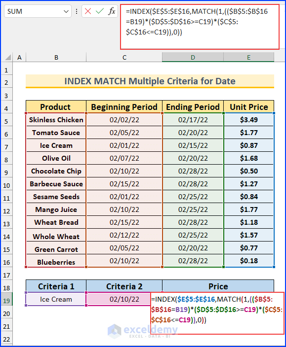
Using INDEX MATCH with Multiple Criteria for Date Range
We want to extract the price for a certain product on a specific date. Suppose we want to see the price of an Ice Cream on 02-10-22 (month-day-year). If the given date falls within the offered period of time, we’ll have the price extracted in any blank cell. Let’s follow the instructions below to use the INDEX MATCH formula with multiple criteria for date range!
Steps:
- Firstly, type the following formula in cell D19.
=INDEX($E$5:$E$16,MATCH(1,(($B$5:$B$16=B19)*($D$5:$D$16>=C19)*($C$5:$C$16<=C19)),0))
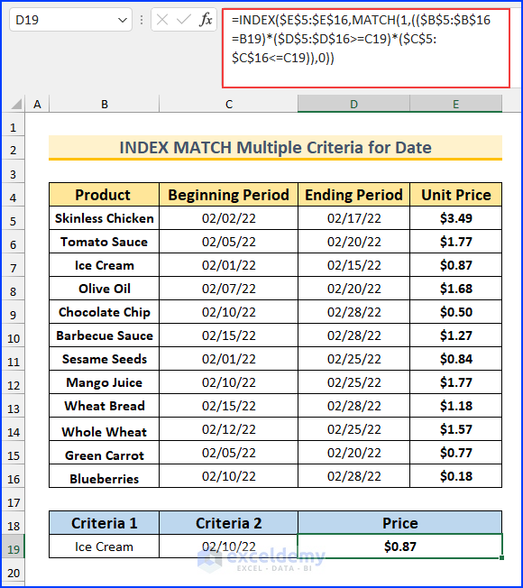
- Then, press Enter if you are using Microsoft 365. However, if you are using older versions of Excel, then press Ctrl+Shift+Enter.
Formula Breakdown
- Firstly, in the formula, $E$5:$E$16 refers to the array argument. Inside the MATCH function $B$5:$B$16=B19, $D$5:$D$16>=C19, and $C$5:$C$16<=C19 declare the criteria.
- Secondly, the MATCH function locates the position of a given value within a row, column, or table. As we said earlier, the MATCH portion passes the row number for the INDEX function.
- Thirdly, the MATCH portion assigns 1 as lookup_value, ($B$5:$B$16=G5)*($D$5:$D$16>=H5)*($C$5:$C$16<=H5) as lookup_array, and 0 declares the [match_type] as an exact match.
- Finally, the used MATCH formula returns 3 as it finds Ice Cream in row number 3.
Download Practice Workbook
You can download the Excel file from the link below.
Conclusion
We have shown you two quick methods of how to use the INDEX and MATCH functions for multiple criteria without an array in Excel. So, using these methods, you can find any data matching multiple criteria from any data set. This is pretty convenient. Do you know any other methods? Let us know in the comment section.
<< Go Back to Multiple Criteria | INDEX MATCH | Formula List | Learn Excel
Get FREE Advanced Excel Exercises with Solutions!

Filters on each column you can specify equal to less than or greater than super handy!
Thanks, James!
Thank you for this. I was looking to see how to use the non-array version in LibreOffice Calc as opposed to Excel and found that it works when you change the formula from (as you have written it):
=INDEX(B5:B24,MATCH(1,INDEX((C5:C24=100)*(D5:D24=100)*(E5:E24=100),0,1),0),1)
To:
=INDEX(B5:B24,MATCH(1,INDEX((C5:C24=100)*(D5:D24=100)*(E5:E24=100),0,0),0),1)
It worked. For some reason, the “1” just before the third to last parenthesis throws it off in Calc. It may be a bug in Calc for LO 7.4.
I checked the last Excel version I own (2010) and it worked with either the “1” or “0” in that space.
Paul, we appreciate your analysis. That 1 represents column_number, which is an optional argument. You can omit that in the original formula and it will still return Ricky Ben.
=INDEX(B5:B24,MATCH(1,INDEX((C5:C24=100)*(D5:D24=100)*(E5:E24=100),0),0),1)