Sometimes, it is important to mark cells in Excel that have some specific values. Most often, users need to differently mark negative and positive values. By doing this, we can read the data easily. In this article, we will see some easy ways to make negative numbers red in Excel.
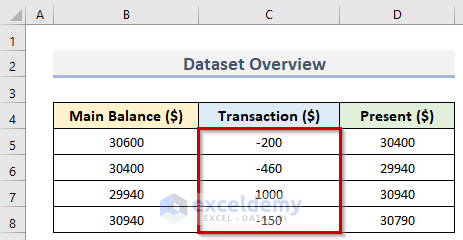
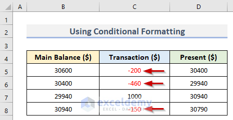
Here, we will demonstrate 4 easy ways to make negative numbers red in Excel. For this, we have used a dataset (B4:D8) in Excel that contains the Main Balance, Transaction and Present Balance. We can see 3 negative numbers in cells C5, C6, and C8 respectively. Now, we will make these negative numbers red by using some features in Excel. So, without further delay, let’s get started.
1. Using Conditional Formatting to Make Negative Numbers Red in Excel
You can highlight cells in Excel with any specific color based on the value of the cell using Conditional Formatting. In this method, we will apply the Conditional Formatting option in Excel for presenting the negative numbers (C5, C6, C8) in red color. However, we can do this very easily by following the quick steps below.
Steps:
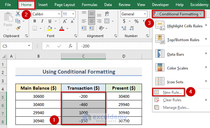
- First, select the range (C5:C8) where you want to apply Conditional Formatting.
- Secondly, go to the Home tab.
- Thirdly, click on the Conditional Formatting dropdown in the Styles group.
- Now, select New Rule from the dropdown.
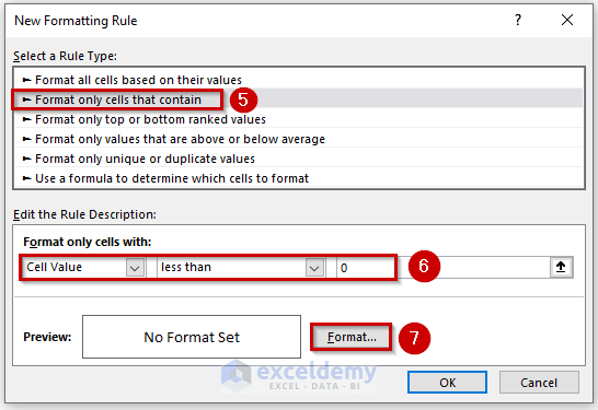
- In turn, the New Formatting Rule dialog box will pop up.
- Next, click on ‘Format only cells that contain’ from the Select a Rule Type section.
- Then, go to the Format only cells with section and select Cell Value and less than for the first two sections from the dropdown.
- After that, put your cursor in the third section and type 0.
- Eventually, click on Format to mention the font color.
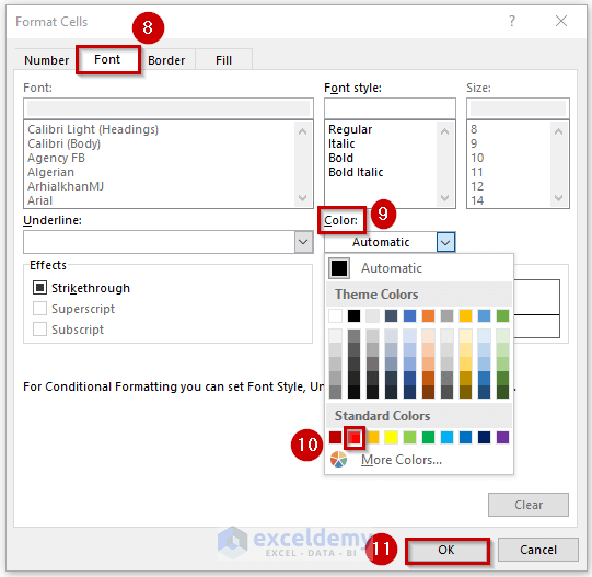
- Therefore, the Format Cells dialog box will appear.
- Afterward, go to the Font tab > Color > Red > OK.
- See the screenshot below for a better understanding.
- After clicking the OK button, we can see the red font color in the Preview section.
- Finally, click OK to apply the formatting in the selected range (C5:C8).

- Consequently, we can see the negative numbers in cells C5, C6 and C8 in red color.
Read More: How to Add Brackets to Negative Numbers in Excel
2. Showing Negative Numbers in Red with Built-In Excel Functionality
Here, we will apply the built-in function in Excel to display the negative numbers in cells C5, C6 and C8 as red. This built-in function is available in the Number group of the Home tab. Follow the steps below to apply this method.
Steps:
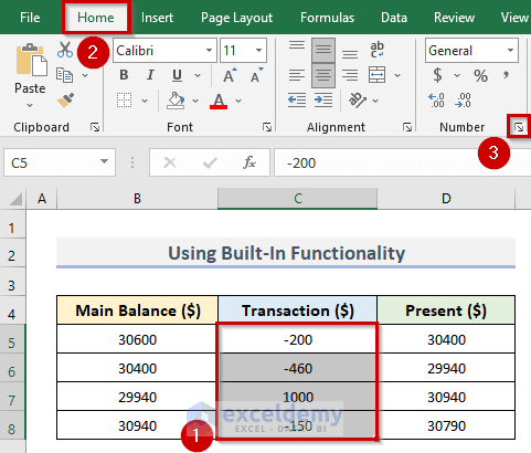
- In the beginning, select the specific range (C5:C8) where you have the negative numbers.
- After that, go to the Home tab.
- Next, go to the Number group and click on the Number Format dialog launcher.
- See the location of the Dialog launcher in the picture below.
- As a consequence, the Format Cells dialog box will show up.
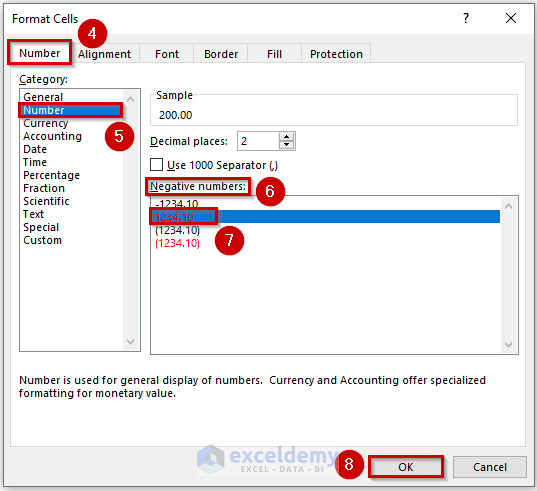
- Accordingly, go to the Number tab.
- Now, select Number from the Category section.
- Then, go to the Negative numbers section.
- Subsequently, select the number with red color.
- In the end, click OK.
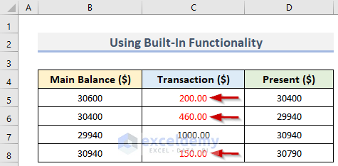
- In this way, we can make the negative numbers red.
Read More: Excel Negative Numbers in Brackets and Red
3. Creating Custom Number Format to Mark Negative Numbers with Red Color
If a built-in number format does not satisfy your requirements, you can create a custom number format. In this method, we will learn to create a custom number format to make negative numbers red. Let’s see the steps below.
Steps:
- In the first place, select the desired range (C5:C8).
- Later, go to the Home tab > click on the Number Format dialog launcher.
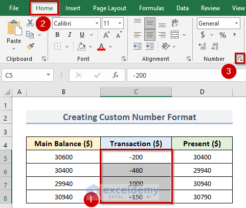
- As a result, we will see the Format Cells dialog box.
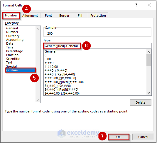
- Eventually, go to the Number tab.
- Then, select Custom in the Category section.
- Now, keep the cursor in the box below Type.
- Therefore, enter the following code in the box:
General;[Red]-General
- Lastly, click the OK button.
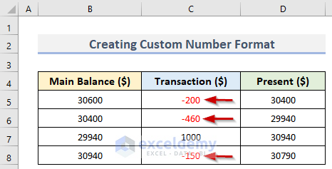
- Thus, all the negative numbers of the selection are expressed in red color.
Read More: How to Put Negative Percentage Inside Brackets in Excel
4. Applying Excel VBA to Make Negative Numbers Red
VBA is Excel’s programming language that is used for numerous time-consuming activities. Here, we will use the VBA code in Excel to show the negative numbers in red color. While applying the VBA code you need to be very careful of the steps. Because, if you miss any step then the code will not run. The steps are below.
Steps:
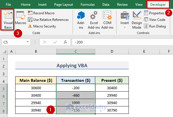
- To begin with, select the range (C5:C8) of Transaction.
- Now, to open the VBA window, go to the Developer tab.
- Therefore, click on Visual Basic.
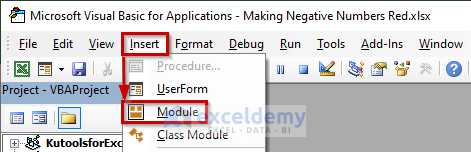
- Hence, the Microsoft Visual Basic for Applications window will open up.
- Then, click on Insert and select Module.
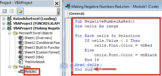
- Accordingly, the Module1 window will appear.
- Next, insert the following code in the window:
Sub NegativeNumberAsRed()
Dim cells As range
For Each cells In Selection
If cells.Value < 0 Then
cells.Font.Color = vbRed
Else
cells.Font.Color = vbBlack
End If
Next cells
End Sub- You must keep the cursor in the last line of the code (see the screenshot below) before running the code.
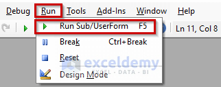
- Eventually, click on Run and select Run Sub/UserForm.
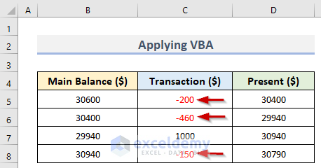
- After running the code, we will see the negative numbers in red color just like the picture below.
Download Practice Workbook
Download the practice workbook from here.
Conclusion
I hope the above methods will be helpful for you to make negative numbers red in Excel. Download the practice workbook and give it a try. Let us know your feedback in the comment section.
Related Articles
- How to Convert Negative Value to Positive in Excel Using Formula
- Excel Formula for Working with Positive and Negative Numbers
- How to Move Negative Sign at End to Left of a Number in Excel
- How to Put Parentheses for Negative Numbers in Excel
- How to Sum Negative and Positive Numbers in Excel
- How to Change Positive Numbers to Negative in Excel
<< Go Back to Negative Numbers in Excel | Number Format | Learn Excel
Get FREE Advanced Excel Exercises with Solutions!
