How to Use the INDIRECT Function to Get Values from Different Sheet in Excel (5 Practical Cases)

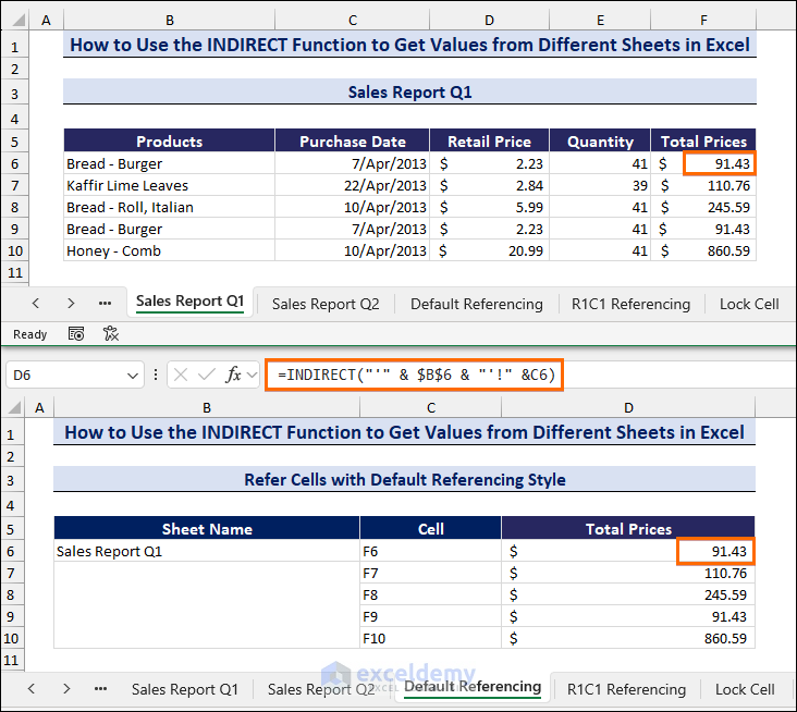
In the following image, we have Sheet Names, Cell references, and their Total Prices. In cell B6, we entered the sheet names (e.g., Sales Report Q1) and inserted the cell references in the Cell column. Then, in the Total Prices column, we applied a formula with the INDIRECT function. The INDIRECT function takes the B6 text value as a sheet name reference and searches the F6 cell of that sheet. In cell D6, it returns the value of the F6 cell in the Sales Report Q1 worksheet.

Excel INDIRECT Function

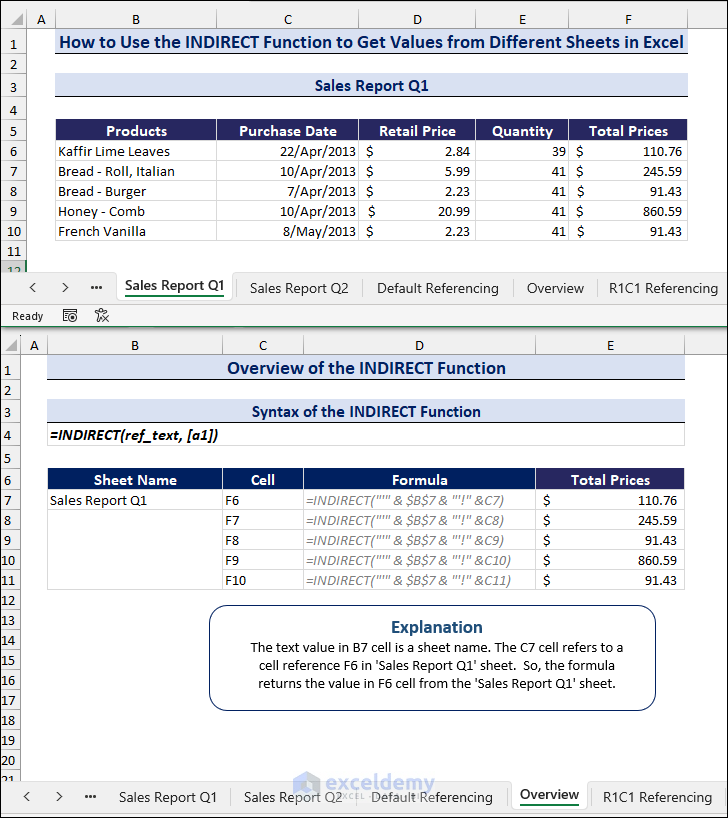
The INDIRECT function returns references according to the text value. It takes the value as a string (ref_text) and returns the reference(s) with that name. These references can be cells, named ranges, or worksheets.

Syntax

This function is a volatile function, which means that each time you open the workbook, it recalculates the data. One of the most useful aspects of the INDIRECT function is that when you insert new rows or columns, it won’t change its reference. Similarly, references won’t change when you remove the existing ones.
In the image below, you can get an overview of the INDIRECT function.

Case 1 – Use INDIRECT Function to Dynamically Refer Cells Across Different Sheets in Excel

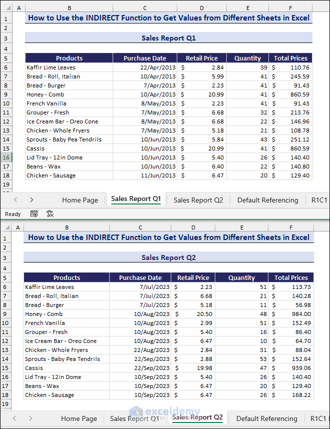
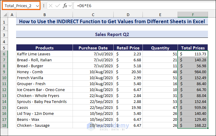
We will use two sample data sets in two different sheets named Sales Report Q1 and Sales Report Q2.

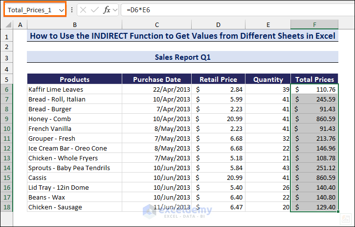
In the following data sets, we have collected the sales details for the first quarter (April, May, and June) and the second quarter (July, August, and September). The image below shows the two datasets, with the products’ names varying with their purchase dates, retail prices, and quantities.

Method 1.1 Refer Cells with Default Referencing Style

In this section, we will refer to cells with default referencing cell style from different sheets (e.g., Sales Report Q1) and get data in a new sheet.

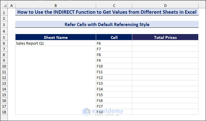
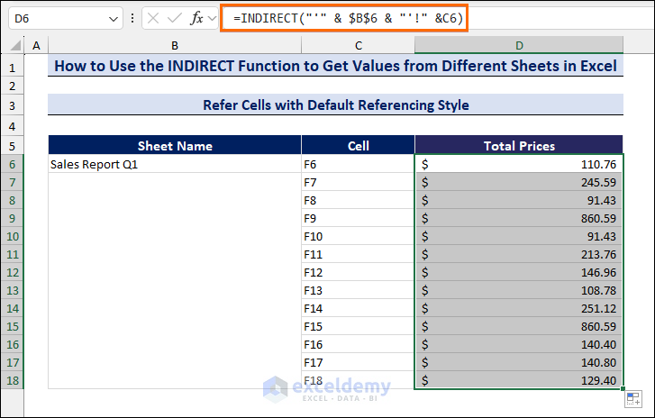
Here, we have taken cell references from F6 to F18 to find the total prices of different quarters:

• Copy the following formula to cell D6:

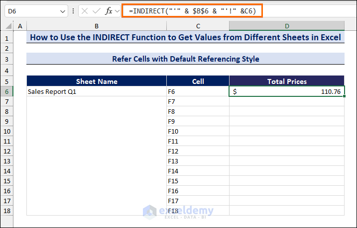
• Press Enter and use the Fill handle to copy the formula to other cells in the column.

• We have created a data validation drop-down list to select the sheets.
• Change the sheet name in the drop-down list and get the values from different sheets.

Method 1.2 Refer Cells with R1C1 Referencing Style

We will use the R1C1 referencing style, which refers to row number and column number (e.g. F6 cell means row 6, column 6). In column C and column D, we have taken all the cell references in R1C1 format.

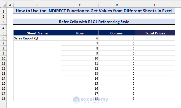
• In cell D6, enter the following formula:

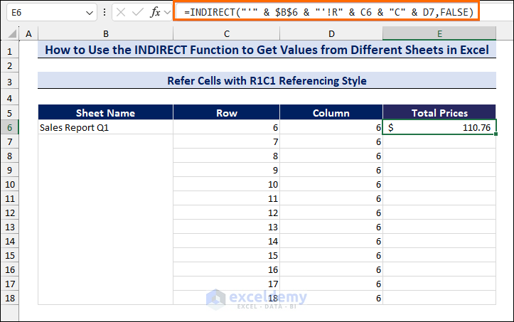
• Press Enter and drag the Fill handle to copy the formula.

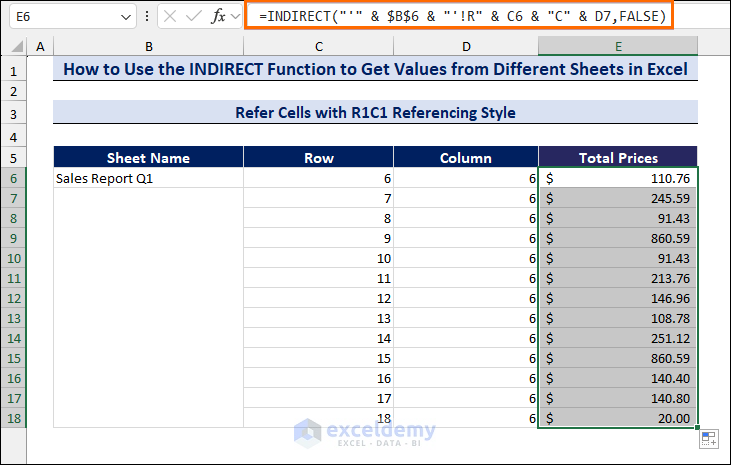
• We have created a drop-down list to select the sheets.
• Change the sheet name in the drop-down list and get the values from different sheets.

Read More: Create Drop-Down List Using INDIRECT Function in Excel

Case 2 – Extract a List of Values with INDIRECT Function from Different Sheets Using Named Range

• Create a Named Range (Total_Prices_1) with the Total Prices column in the sheet Sales Report Q1.

• Create a Named Range (Total_Prices_2) with the Total Prices column in the sheet Sales Report Q2.

• To get the total prices for the first quarter from the Sales Report Q1 sheet, enter the following formula in cell D6 and press Enter.

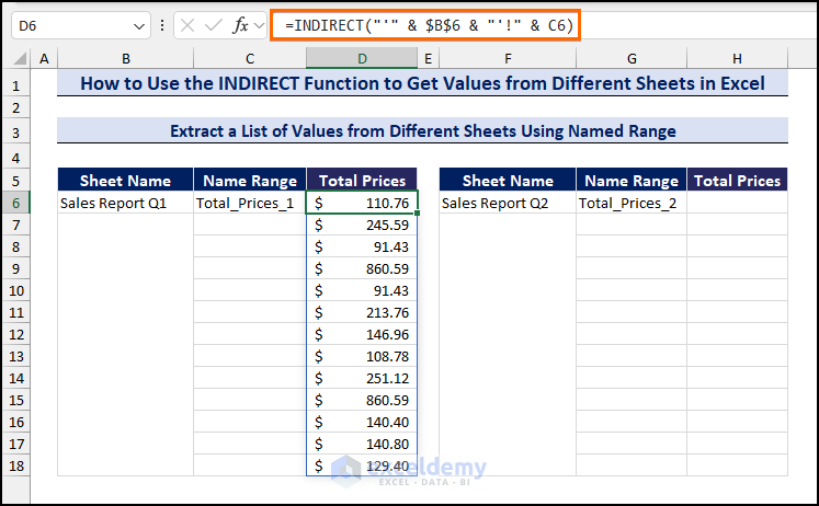
• To get the total values for the second quarter from the Sales Report Q2, insert the following formula in cell H6:

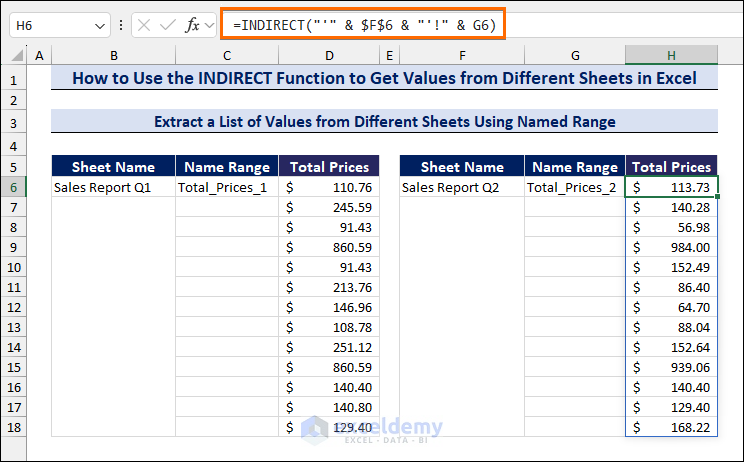
Read More: INDIRECT Function with Sheet Name in Excel

Case 3 – Lock Cell References with INDIRECT Function to Prevent Automatic Formula Changes Across Different Sheets

The INDIRECT function can lock cell references. It helps avoid errors when the cell reference changes while adding or removing rows or columns.

From our example, we will calculate the total prices from the sheet Sales Report Q1 by using the SUM and INDIRECT functions. Then, we will calculate the same total using only the SUM function. Then, we will insert a new row in the source sheet, Sales Report Q1.

We will see that a formula using the INDIRECT function gives the newly updated total, but using only the SUM function will not result in an updated total. Follow the steps below to see it in action:

• In cell D6, enter the following formula in the Sales Report Q1 sheet to get the Total Prices column.

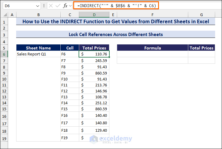
• Calculate the Total Prices with the following formula in cell G6:

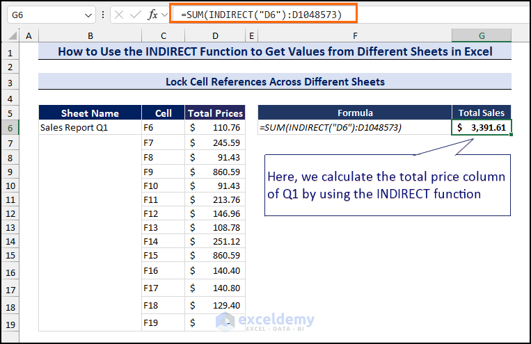
• We will again calculate the Total Prices of Sales Report Q1 column with the SUM function in cell G7:

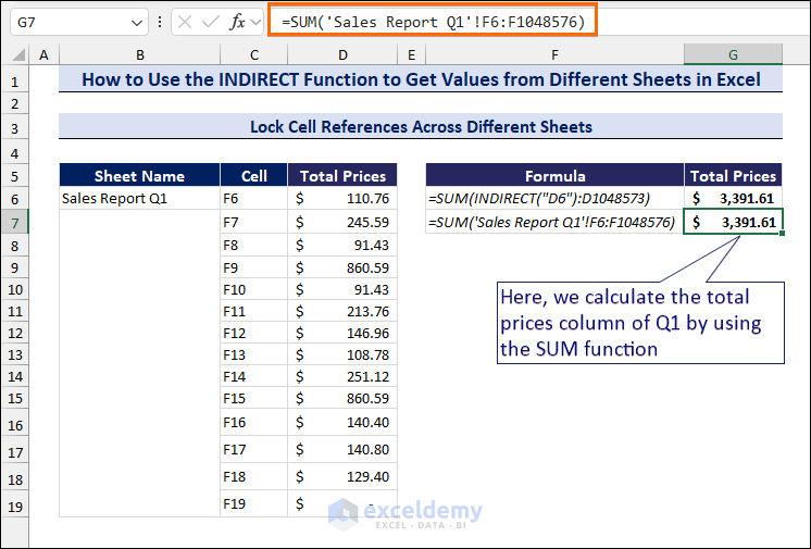
• Insert a new row in the Sales Report Q1 sheet.
• You can see that the G6 cell has been updated with the new total of $3,483.04, but the G7 cell has remained the same at $3,391.61.

Read More: How to Use Excel INDIRECT Range

Case 4 – Create a Drop-Down List and Analyze Data from Different Sheets with INDIRECT Function in Excel

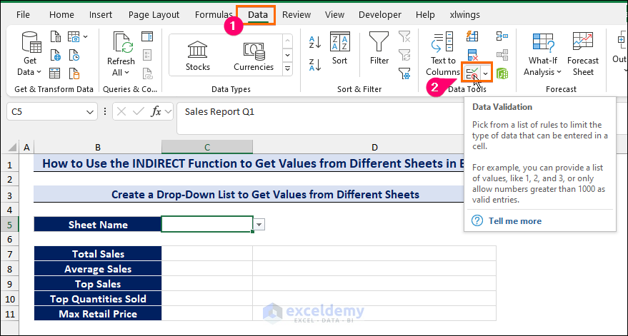
• Select cell C5 where you want to create the drop-down list with the sheet names.
• Go to the Data tab.
• Click on the Data Validation command from the Data Tools group.

Click on the image to see the full view

• From the Data Validation dialog box, go to the Settings tab.
• Select the List option for the Allow criteria.
• Type the names of the sheets Sales Report Q1, Sales Report Q2 in the Source criteria.
• Click OK.

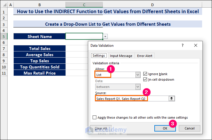
• You will get your data validation drop-down list in cell C5.

We will assign formulas to calculate the total sales, average sales, top sales, top quantities sold, and maximum retail prices of a selected sheet from the drop-down list (cells C7 to C11):

• Formula to calculate the total sales, C7:

• Formula to calculate the average sales, C8:

• Formula to calculate the top sales, C9:

• Formula to calculate the top quantities sold, C10:

• Formula to calculate the maximum retail price, C11:

• Choose any of the sheet names from the drop-down list and get your analytical data from different sheets.

Read More: How to Convert Text to Formula Using the INDIRECT Function in Excel

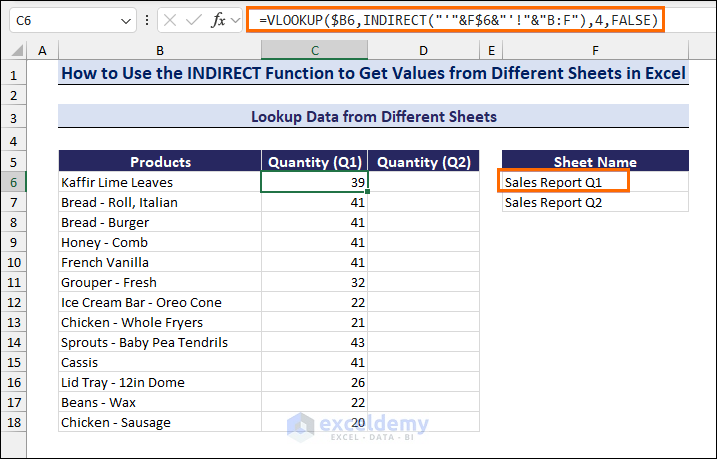
Case 5 – Lookup Data from Different Sheets in Excel with INDIRECT and VLOOKUP Functions

The benefit of using the VLOOKUP function here is that we do not need to specify the cell reference in the INDIRECT function. The INDIRECT function takes a table range (e.g., B:F). So, we can get any value from the table range just by changing its column index number in the VLOOKUP function. We can find total sales, quantities, purchase dates, or any other parameters only by changing the column index number:

• To get the sold quantities in the first quarter, enter the following formula in cell C6:

• Drag down the Fill handle to copy the formula along the Quantity (Q1) column.

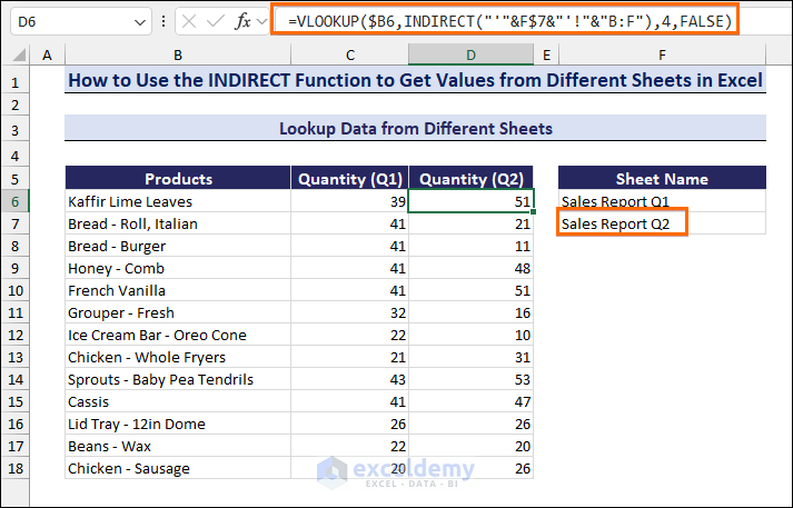
• To get the quantities sold in the second quarter, enter the following formula in the D6 cell:

• Drag down the Fill handle to copy the formula along the Quantity (Q2) column.

Read More: How to Use Indirect Address in Excel

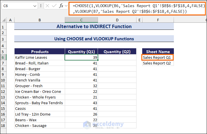
An Alternative to INDIRECT Function: CHOOSE and VLOOKUP Functions

• Enter the following formula in cell C6 to get the value of sold quantities in the first quarter:

• Drag down the Fill handle to copy the formula along the Quantity (Q1) column.

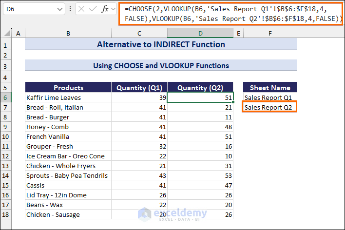
• Enter the following formula in cell D6 to get the value of sold quantities in the second quarter:

• Drag down the Fill handle to copy the formula along the Quantity (Q2) column.

Download Practice Workbook

<< Go Back to Excel INDIRECT Function | Excel Functions | Learn Excel