Excel 365 provides us with a powerful function for automatically filtering our datasets, named the FILTER function. It makes our task easier by using this function in Excel formulas. This article will share the complete idea of how the FILTER function works in Excel independently and then with other Excel functions. If you are also curious about it, download our practice workbook and follow us.
Introduction to the FILTER Function in Excel
Function Objective:
Filter some particular cells or values according to our requirements.
Syntax:
=FILTER (array, include, [if_empty])Arguments Explanation:
| Argument | Required or Optional | Value |
|---|---|---|
| array | Required | An array, an array formula, or a reference to a range of cells for which we require the number of rows. |
| include | Required | This works like a Boolean array; it carries the condition or criteria for filtering. |
| [if_empty] | Optional | Pass the value to return when no results are returned. |
Return Parameter:
The function returns a dynamic result. When values in the source data change, or the source data array is resized, the results from FILTER will update automatically.
How to Use the FILTER Function in Excel: 10 Ideal Examples
To demonstrate the examples, we consider a dataset of 10 students of an institution. Their ID, name, department, enrolled semester, and the amount of CGPA are in the range of cells B5:F14.
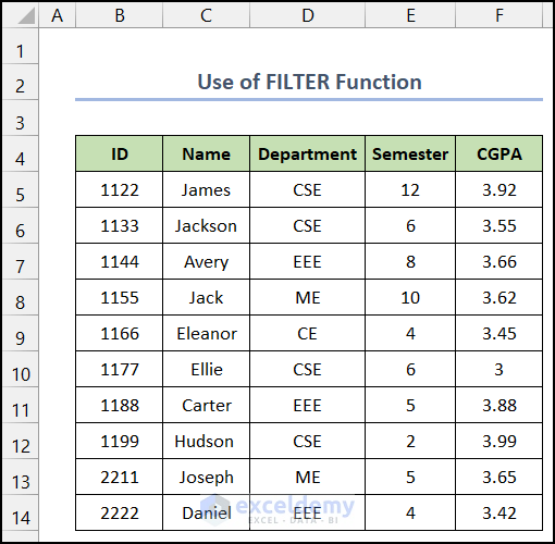
📚 Note:
All the operations of this article are accomplished by using the Microsoft Office 365 application.
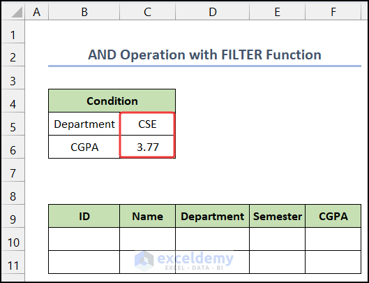
1. Performing AND Operation with FILTER Function for Multiple Criteria
In the first example, we will perform the AND operation by the FILTER function. Our desired conditions are in the range of cells C5:C6.
The steps to complete this example are given below:
📌 Steps:
- First of all, select cell B10.
- Now, write down the following formula in the cell.
=FILTER(Dataset!B5:F14,(Dataset!D5:D14=C5)*(Dataset!F5:F14>=C6),"no results")
- Then, press Enter.
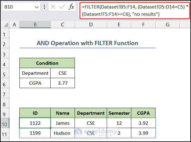
- You will get the filtered result in the range of cells B10:F11.
Thus, we can say that we are able to apply the FILTER function for the AND operation.
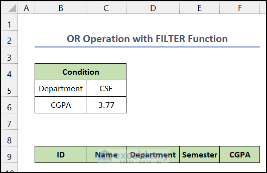
2. Application of OR Operation with FILTER Function for Multiple Criteria
In the second example, we are going to use the FILTER function for the OR operation. Here, we mentioned the conditions in the range of cells C5:C6.
The steps to finish this example are given as follows:
📌 Steps:
- First, select cell B10.
- After that, write down the following formula in the cell.
=FILTER(Dataset!B5:F14,(Dataset!D5:D14=OR!C5)+(Dataset!F5:F14>=OR!C6),"no results")
- Press Enter.
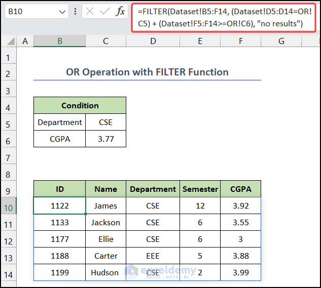
- You will figure out the filtered result in the desired cells.
Hence, we are able to use the FILTER function perfectly for the OR operation.
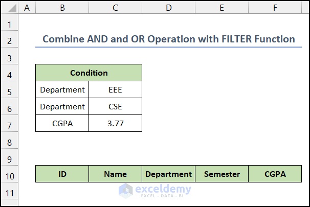
3. Combination of AND and OR Logic with FILTER Function
Now, we will use the FILTER function for a combined AND and OR operation. The conditions are in the range of cells C5:C7.
The steps to accomplish this example are given below:
📌 Steps:
- At first, select cell B11.
- Afterward, write down the following formula in the cell.
=FILTER(Dataset!B5:F14,(Dataset!F5:F14>=Combine!C7)*((Dataset!D5:D14=Combine!C5)+(Dataset!D5:D14=Combine!C6)),"No results")
- Press the Enter.
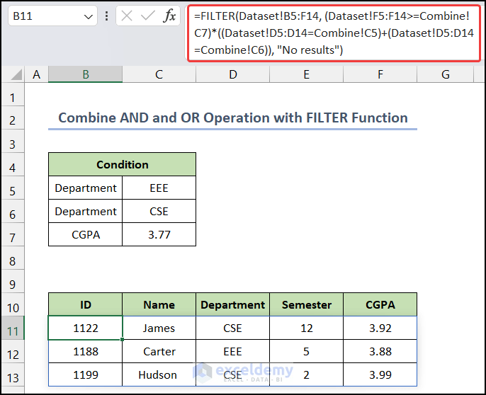
- You will notice the filtered result will be available in the cells.
Therefore, our formula works effectively and we are able to perform the AND and OR operations simultaneously by the FILTER function.
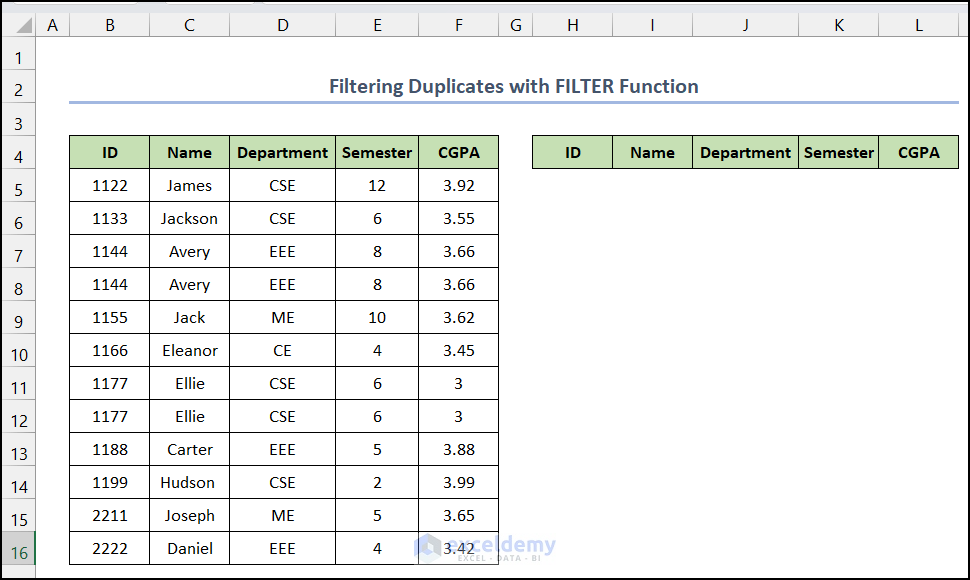
4. Filtering Duplicates Using FILTER Function
In this example, we are going to filter out the duplicate entities from our dataset. Our dataset contains 2 duplicate entities.
The steps of this example are given below:
📌 Steps:
- In the beginning, select cell H5.
- Next, write down the following formula in the cell.
=FILTER(B5:F16,COUNTIFS(B5:B16,B5:B16,C5:C16,C5:C16,D5:D16,D5:D16,E5:E16,E5:E16,F5:F16,F5:F16)>1,"No result")
- Thus, press the Enter.
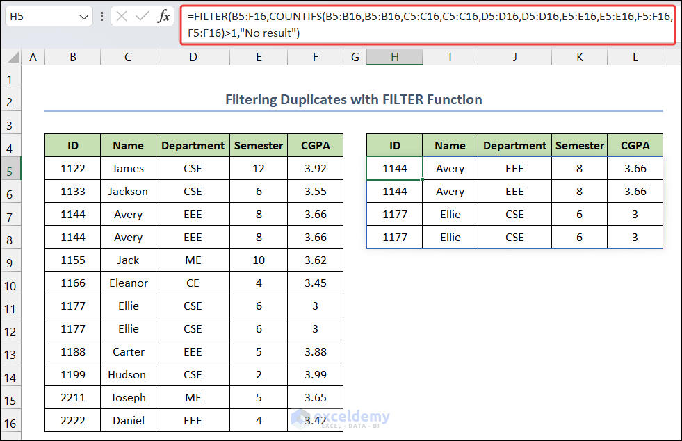
- You will see that all the duplicate values are listed separately.
At last, we can say that our formula works precisely and we are able to figure out the duplicates by the FILTER function in Excel.
🔎 Explanation of the Formula
👉 COUNTIFS(B5:B16,B5:B16,C5:C16,C5:C16,D5:D16,D5:D16,E5:E16,E5:E16,F5:F16,F5:F16): The COUNTIFS function checks the presence of the duplicate values.
👉 FILTER(B5:F16,COUNTIFS(B5:B16,B5:B16,C5:C16,C5:C16,D5:D16,D5:D16,E5:E16,E5:E16,F5:F16, F5:F16)>1,”No result”): Finally, the FILTER function filter the duplicate values and listed them separately.
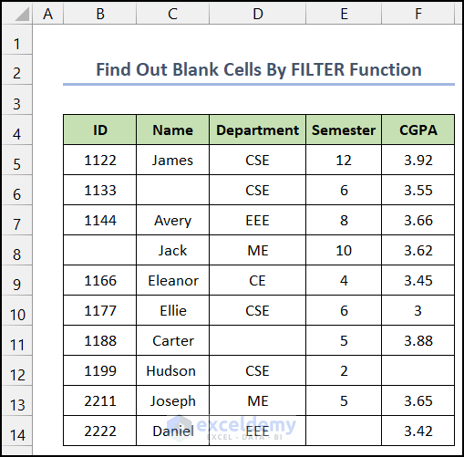
5. Find Out Blank Cells by FILTER Function
We have a dataset with some blank cells. Now, we are going to filter out the cells that don’t contain any blank function with the help of the FILTER function.
The procedure to filter out the complete rows is given below::
📌 Steps:
- Firstly, select cell H5.
- Next, write down the following formula in the cell.
=FILTER(B5:F14,(B5:B14<>"")*(C5:C14<>"")*(D5:D14<>"")*(E5:E14<>"")*(F5:F14<>""),"No results")
- After that, press Enter.
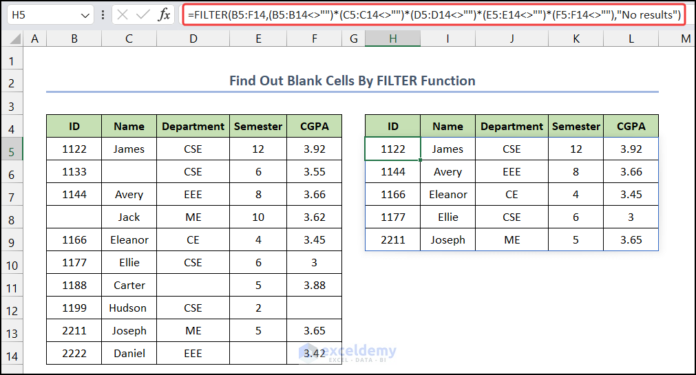
- You will get those entities that don’t have any blank cells.
So, we can say that our formula works fruitfully and we are able to get the value with no blank cells by the Excel FILTER function.
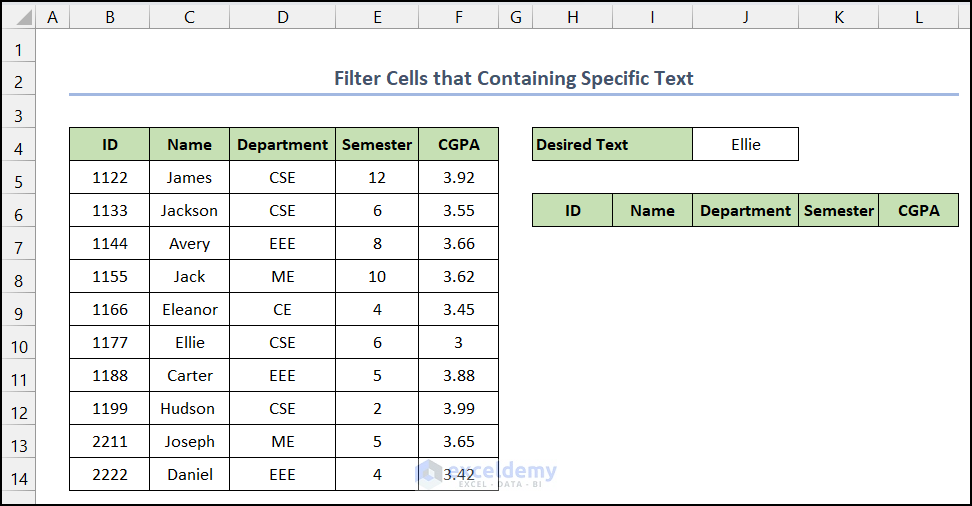
6. Filter Cells That Contain Specific Text
Using the FILTER function, we can easily search for any particular value and filter out the corresponding entities from our original dataset. Besides the FILTER function, the ISNUMBER and SEARCH functions also help us to complete the formula. Our desired text ‘Ellie’ is displayed in cell J4.
The approach of filtering out the data for a specific text is described below::
📌 Steps:
- At the start, select cell H7.
- Then, write down the following formula in the cell.
=FILTER(B5:F14,ISNUMBER(SEARCH(J4,C5:C14)),"No results")
- Next, press the Enter key.
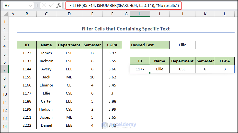
- You will get the result with that particular text.
Thus, we are able to apply the formula successfully and get the value for our specific text value.
🔎 Explanation of the Formula
👉 SEARCH(J4,C5:C14): The SEARCH function will return the cells which will be matched with the input value.
👉 ISNUMBER(SEARCH(J4,C5:C14)): The ISNUMBER function will return true if the search value is a number other than false.
👉 FILTER(B5:F14,ISNUMBER(SEARCH(J4,C5:C14)),”No results”): Finally, the FILTER function extracts the matched rows and shows them.
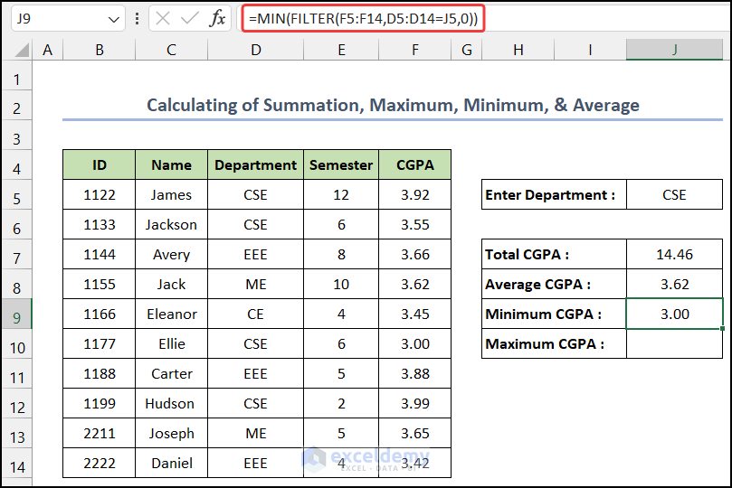
7. Calculation of Summation, Maximum, Minimum, and Average
Now, we are going to perform some mathematical calculations with the help of the FILTER function. The data for which we will filter will be in cell J5. Here, we are going to determine all the values for the CSE department.
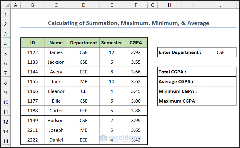
Besides the FILTER function, the SUM, AVERAGE, MIN, and MAX functions will be used for completing the evaluation process. The estimated value will be in the range of cells J7:J10. The calculation procedure is explained below step-by-step:
📌 Steps:
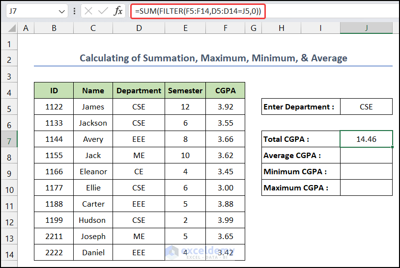
- First of all, select cell J7.
- Now, write down the following formula in the cell for the summation.
=SUM(FILTER(F5:F14,D5:D14=J5,0))
🔎 Explanation of the Formula
👉 FILTER(F5:F14,D5:D14=J5,0): The FILTER function filters the CGPA value of our desired department.
👉 SUM(FILTER(F5:F14,D5:D14=J5,0)): Finally, the SUM function adds all of them.
- Press Enter.
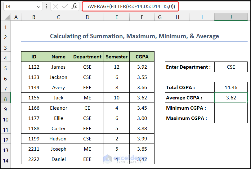
- After that, select cell J8, and write down the following formula for the average value.
=AVERAGE(FILTER(F5:F14,D5:D14=J5,0))
🔎 Explanation of the Formula
👉 FILTER(F5:F14,D5:D14=J5,0): The FILTER function filters the CGPA value of our desired department.
👉 AVERAGE(FILTER(F5:F14,D5:D14=J5,0)): The AVERAGE function will calculate the average value of those values.
- Again, press Enter.
- Then, select cell J9, and write down the following formula inside the cell for getting the minimum value.
=MIN(FILTER(F5:F14,D5:D14=J5,0))
🔎 Explanation of the Formula
👉 FILTER(F5:F14,D5:D14=J5,0): The FILTER function filters the CGPA value of our desired department.
👉 MIN(FILTER(F5:F14,D5:D14=J5,0)): The MIN function will figure out the minimum value among the 4 values.
- Similarly, press the Enter.
- Finally, select cell J10, and write down the following formula inside the cell for the maximum value.
=MAX(FILTER(F5:F14,D5:D14=J5,0))
🔎 Explanation of the Formula
👉 FILTER(F5:F14,D5:D14=J5,0): The FILTER function filters the CGPA value of our desired department.
👉 MAX(FILTER(F5:F14,D5:D14=J5,0)): The MAX function will find out the maximum value among the 4 CGPA values.
- Press Enter for the last time.
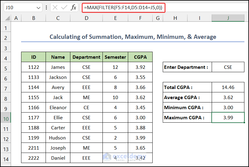
- You will notice all the values for the CSE department will be available.
Hence, we can say that all of our formulas work perfectly, and we are able to get all the desired values by the Excel FILTER function.
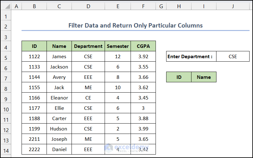
8. Filter Data and Return Only Particular Columns
Here, we are going to use the FILTER function twice in a nested condition to get the particular columns based on our desired value. Our desired entity is in cell J5. We will only show the ID and the Name column.
The steps of this process are given below:
📌 Steps:
- First, select cell H8.
- Then, write down the following formula in the cell.
=FILTER(FILTER(B5:F14,D5:D14=J5),{1,1,0,0,0})
- After that, press Enter.
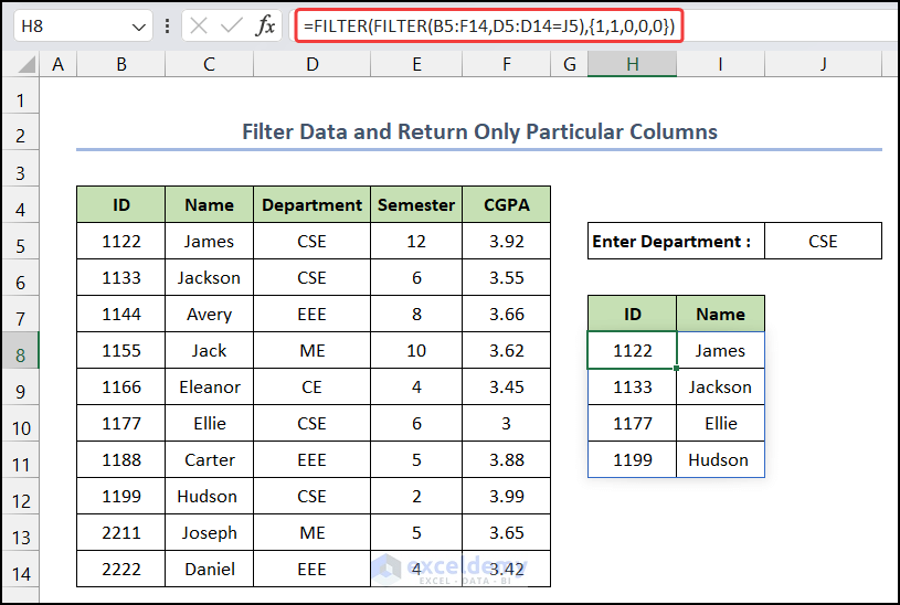
- You will get only the ID and Name column of our desired department.
Therefore, we can say that our formula works properly, and we are able to get some specific columns by the Excel FILTER function.
🔎 Explanation of the Formula
👉 FILTER(B5:F14,D5:D14=J5): The FILTER function will return the matched rows from the given dataset with all the columns.
👉 FILTER(FILTER(B5:F14,D5:D14=J5),{1,1,0,0,0}): The outer FILTER function will select only the first two columns of the selected data. We can either use 0,1 or TRUE, FALSE.
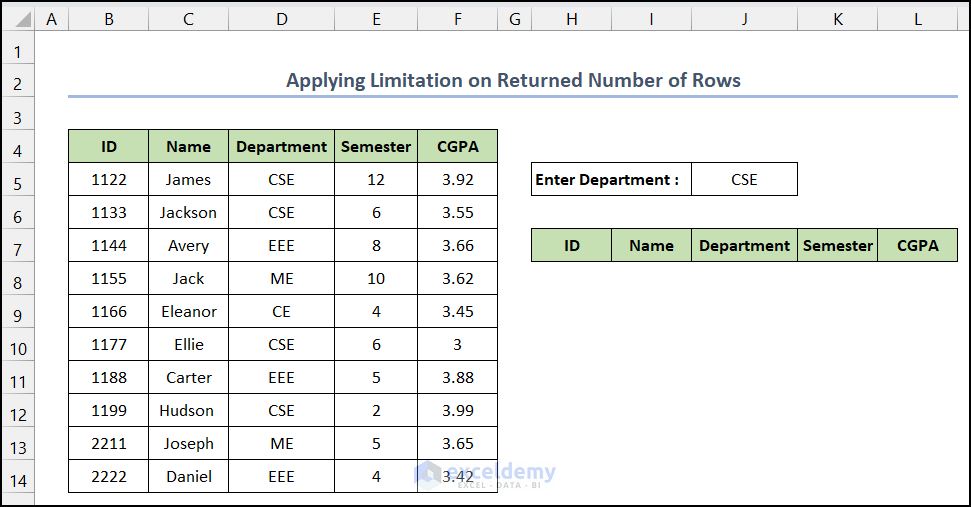
9. Apply Limitation on Returned Number of Rows
In this case, we will add some limitations to the FILTER function for getting the limited number of rows. Our desired department is in cell J5. To apply the limitation, we have to use the IFERROR and INDEX functions also.
The steps of this method are described as follows:
📌 Steps:
- First, select cell H8.
- Next, write down the following formula in the cell.
=IFERROR(INDEX(FILTER(B5:F14,D5:D14=J5),{1;2},{1,2,3,4,5}),"No result")
- Then, press Enter.
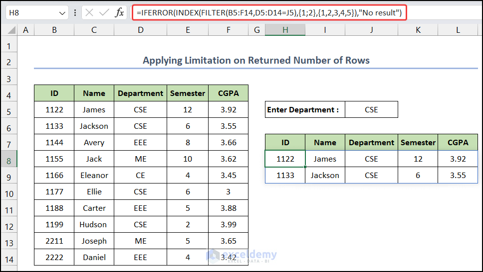
- You will get the result.
So, we can say that we are able to successfully apply the Excel FILTER, INDEX, and IFERROR functions successfully.
🔎 Explanation of the Formula
👉 FILTER(B5:F14,D5:D14=J5): The FILTER function will return the filtered data by matching it with the input value.
👉 INDEX(FILTER(B5:F14,D5:D14=J5),{1;2},{1,2,3,4,5}): This formula will return the first two rows of the matched data. {1;2} This is for the first two rows. And {1,2,3,4,5} this is for selecting the five columns.
👉 IFERROR(INDEX(FILTER(B5:F14,D5:D14=J5),{1;2},{1,2,3,4,5}),”No result”): Lastly, the IFERROR function is used to avoid the error if there is a problem with other function return values.
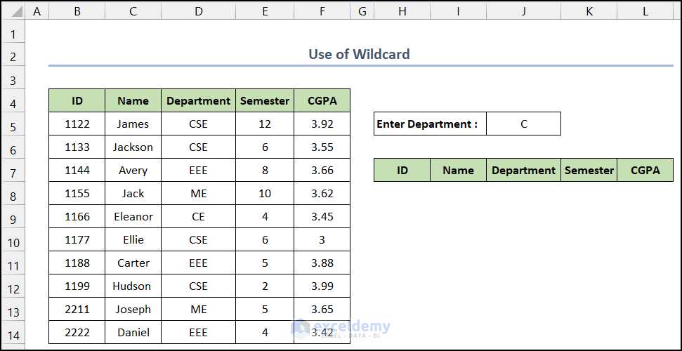
10. Use of Wildcard with FILTER Function
In the last example, we are going to apply the filter wildcard for filtering the data. We will apply the formula with the help of ISNUMBER, SEARCH, and FILTER functions. Our desired value is in cell J5.
The process is explained below step-by-step:
📌 Steps:
- Firstly, select cell H8, and write down the following formula in the cell.
=FILTER($B$5:$F$14,ISNUMBER(SEARCH(J5,D5:D14)),"No Results!")
- Now, press Enter.
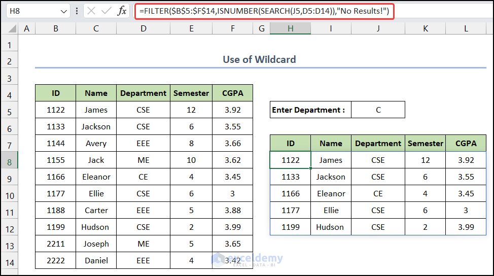
- You will get all the results with the cell value C.
Finally, we can say that our formula works precisely, and we are able to create a wildcard with the Excel FILTER function.
🔎 Explanation of the Formula
👉 SEARCH(J5,D5:D14): The SEARCH function will search the data by matching it with the input value.
👉 ISNUMBER(SEARCH(J5,D5:D14)): This formula will check which result of the SEARCH function is true,
👉 FILTER($B$5:$F$14,ISNUMBER(SEARCH(J5,D5:D14)),”No Results!”): Lastly, the FILTER function will show them in our desired cell.
What Are the Alternatives to the Excel FILTER Function?
From our previous application, you may notice that the Excel FILTER function is a handy function for getting our desired values within a short period of time. There is no specific alternative to this function. However, the combination of some general Excel functions may return us the results of the FILTER function. Among them, the IFERROR, INDEX, AGGREGATE, ROW, ISNA, and MATCH functions are mentionable. But, we recommend that if you have the FILTER function, go for it. The combination of those functions will make the formula more complex to understand others. Besides that, it may slow down your Excel application.
What Are the Possible Reasons If the FILTER Function Does Not Work in Excel?
Sometimes, the FILTER function of Excel doesn’t work properly. Most of the time, it occurs due to the presence of error. Mainly, the #SPILL!, #CALC!, #VALUE! errors usually don’t allow the FILTER function to work, and return the desired data. To eliminate this error, go back to your original dataset and fix it, and you will find that the FILTER function will work smoothly.
The frequently seen errors in Excel are explained below briefly:
| Common Errors | When they show |
|---|---|
| #VALUE | It will appear when the array and include argument have incompatible dimensions. |
| #CALC! | It will appear if the optional if_empty argument is omitted and no results meeting the criteria are found. |
| #NAME | It will appear when trying to use FILTER in an older version of Excel. |
| #SPILL | This error will happen if one or more cells in the spill range are not entirely blank. |
| #REF! | This error will happen if a FILTER formula is used between different workbooks and closes the source workbook. |
| #N/A or #VALUE | This type of error may occur if some value in the included argument is an error or cannot be transformed to a Boolean value (0,1 or TRUE, FALSE). |
Download Practice Workbook
Download this practice workbook for practice while you are reading this article.
Conclusion
That’s the end of this article. I hope that this article will be helpful for you and you will be able to apply the FILTER function in Excel. Please share any further queries or recommendations with us in the comments section below if you have any further questions or recommendations.
<< Go Back to Excel Functions | Learn Excel
Get FREE Advanced Excel Exercises with Solutions!
