Rounding to Nearest Dollar in Excel (6 Easy Ways)

Rounding to the nearest dollar of any price list or any payment list is a pretty common task in our regular life. It provides us with more flexibility in the cash payment system. In this context, we will demonstrate to you 6 different methods of rounding to the nearest dollar in Excel. If you are interested to know about it, download our practice workbook and follow us.

Rounding to Nearest Dollar in Excel: 6 Easy Ways

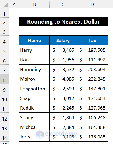
To demonstrate the approaches, we consider a dataset of 10 employees of an institution. The name of the employees are in column B, their salaries per month and the tax payment are in columns C and D respectively. Our dataset is in the range of cells B5:D14. We will be rounding the tax payment to the nearest dollar for the convenience of cash payment, and the final rounded amount will show in column E.

1. Using ROUND Function for Rounding to Nearest Dollar

In this method, we are going to use the ROUND function for rounding to the nearest dollar in Excel. The final result will be in column E. The steps of this method are given below:

📌 Steps:

First of all, select cell E5.
Now, write down the following formula into the cell.

=ROUND(D5,0)

Here, 0 is the num_digits which helps us to round up to the decimal.

Then, press the Enter key.

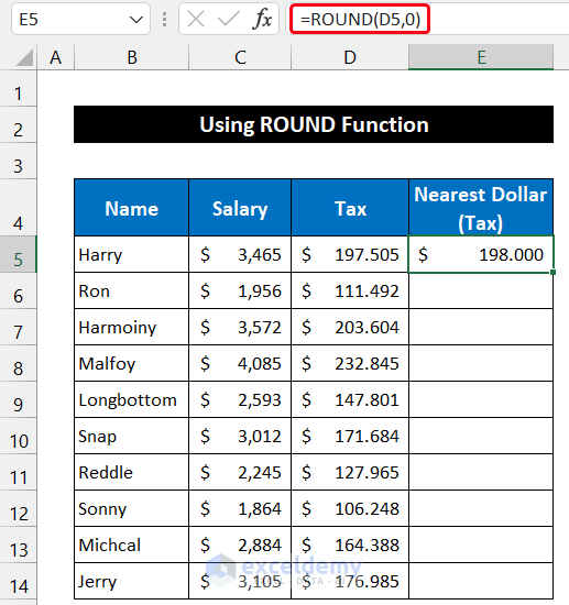
After that, double-click on the Fill Handle icon to copy the formula up to cell E14.

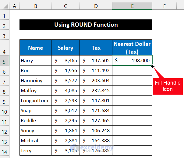
You will see all values were rounding to their nearest round dollar.

Thus, we can say that our formula worked perfectly and we are rounding the tax payment to the nearest dollar.

2. Applying MROUND Function

In this following approach, we will use the MROUND function for rounding to the nearest dollar in Excel. Our dataset is in the ranges of cells B5:D14 and the final result will be in column E. The steps of this process are given below:

📌 Steps:

First, select cell E5.
Then, write down the following formula into the cell.

=MROUND(D5,1)

Here, 1 is the ‘multiple’ value which helps us for rounding to the nearest dollar.

After that, press the Enter key on your keyboard.

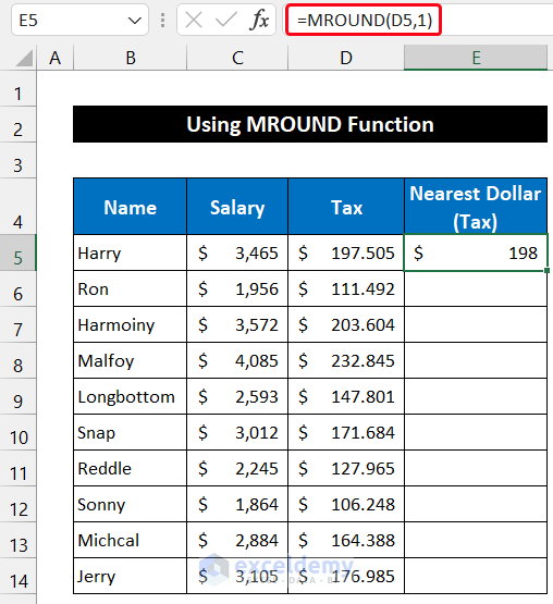
Now, double-click on the Fill Handle icon to copy the formula up to cell E14.

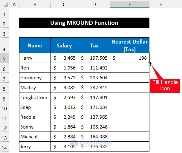
You will get that all values were rounding to their nearest round dollar.

Finally, we can that our formula worked successfully and we are rounding the tax payment to the nearest dollar.

3. Use of ROUNDUP Function

In this process, we will apply the ROUNDUP function for rounding to the nearest dollar in Excel. Our dataset is in the ranges of cells B5:D14 and the final result will be in column E. The procedure of this process is given as follows:

📌 Steps:

At the beginning of this process, select cell E5.
Then, write down the following formula into the cell.

=ROUNDUP(D5,0)

Here, 0 is the num_digits that help us to round up to the decimal.

Press the Enter key to get the result.

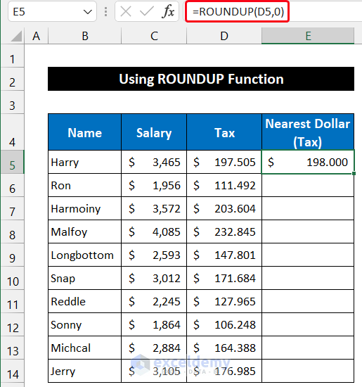
Now, drag the Fill Handle icon with your mouse to copy the formula up to cell E14.

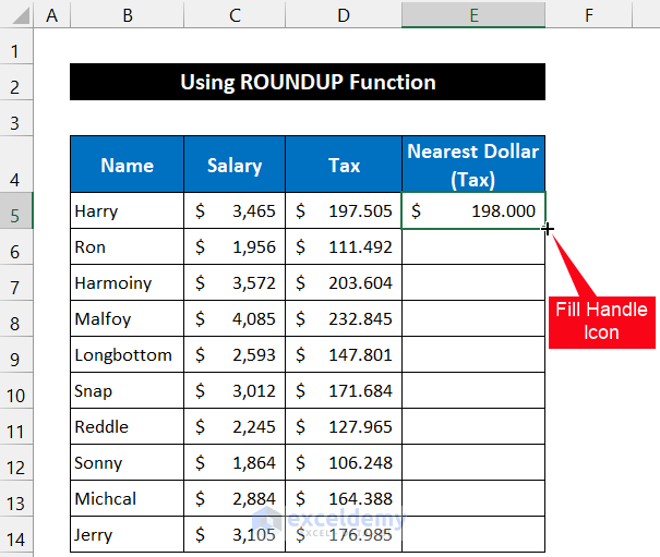
Finally, You will get that all values were rounding to their nearest round dollar.

So, we can that our formula worked precisely and we are rounding the tax payment to the nearest dollar.

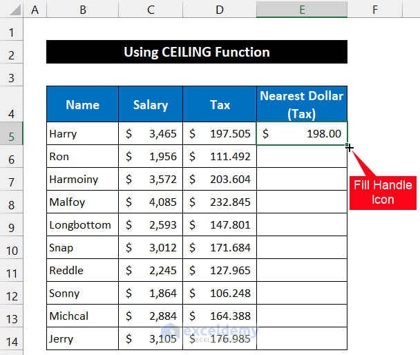
4. Utilizing CEILING Function

In this procedure, the CEILING function will help for rounding to the nearest dollar in Excel. We will show the final result in column E. The approach is explained below:

📌 Steps:

To start up, select cell E5.
After that, write down the following formula into the cell.

=CEILING(D5,1)

Here, 1 is the ‘significance’ value which helps us for rounding to the nearest dollar.

Press the Enter key.

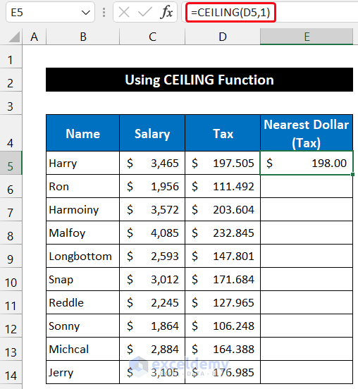
Then, drag the Fill Handle icon with your mouse to copy the formula up to cell E14.

In the end, You will see that all values were rounding to their nearest round dollar.

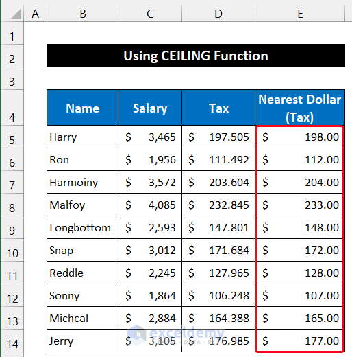
At last, we can that our formula worked effectively and we are rounding the tax payment to the nearest dollar.

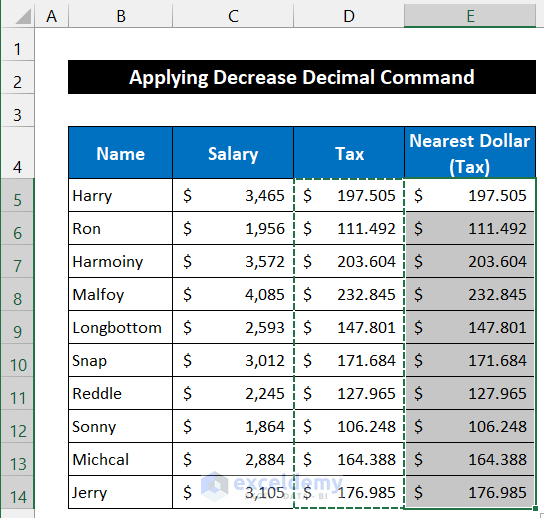
5. Rounding to Nearest Dollar Using Decrease Decimal Command

In the following method, we are going to use the Decrease Decimal command for rounding to the nearest dollar in Excel. We will show the final result in column E, and our dataset is kept in the range of cells B5:D14. The procedure is described below step by step:

📌 Steps:

First, select the entire range of cells D5:D14.
Now, click ‘Ctrl+C’ to copy the data into the Clipboard. As a result, the original payment amount remains intact.
Then, click ‘Ctrl+V’ to paste the data in the range of cell E5:E14.

After that, select the range of cells E5:E14.
In the Home tab, click on the Decrease Decimal command locates in the Number group.

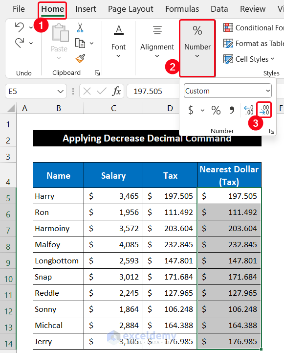
Keep clicking on the command icon until all the digits after the decimal point will disappear.
At last, You will see that all values were rounding to their nearest round dollar.

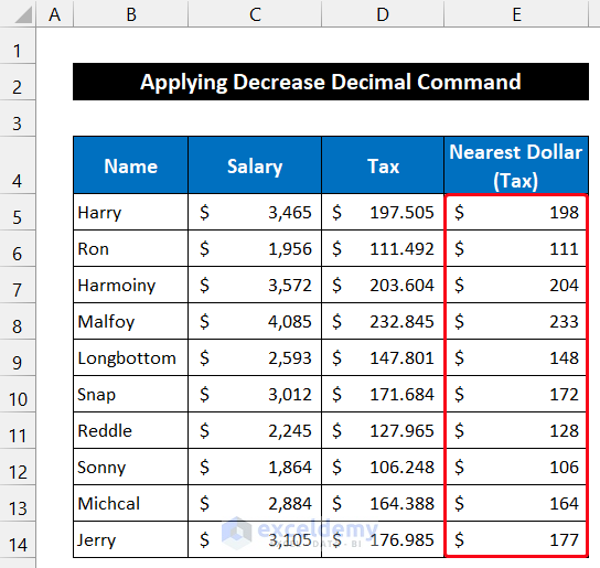
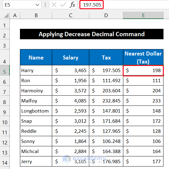
However, if you select any cell in the range E5:E14 and look at the Formula Bar, you can see the whole number like column D.

In the end, we can that our rounding method worked perfectly and we were rounding the tax payment to the nearest dollar.

Read More: Excel VBA: Round to Nearest 5

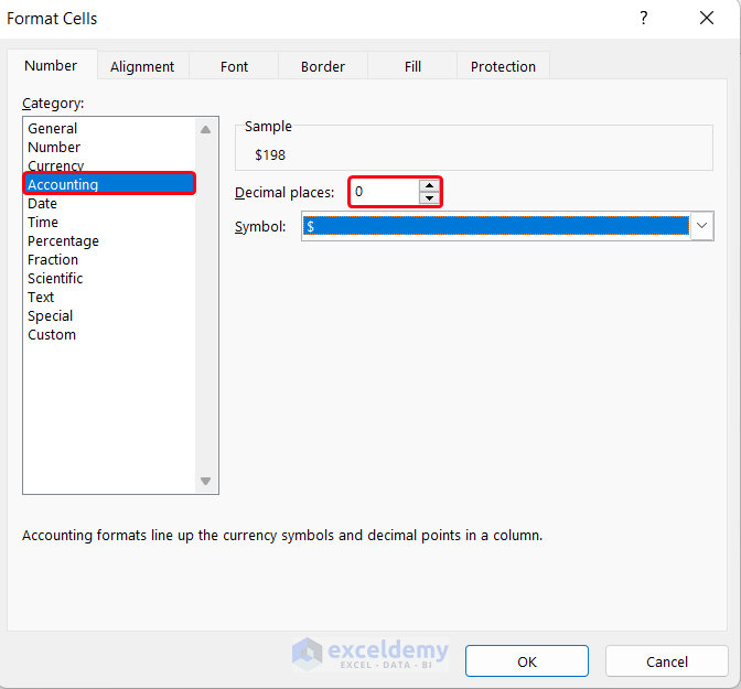
6. Applying Built-in Format Cells Command

In this case, we are going to use the Excel built-in Format Cells command for rounding to the nearest dollar in Excel. Our dataset is kept in the range of cells B5:D14, and we will show the final result in column E. The steps of this approach are given as follows:

📌 Steps:

First of all, select the entire range of cells D5:D14.
Then, click ‘Ctrl+C’ to copy the data into the Excel Clipboard. As a result, our original payment amount will remain unchanged.
After that, click ‘Ctrl+V’ to paste the data in the range of cell E5:E14.

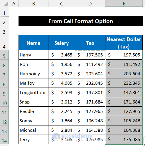
Now, select the range of cells E5:E14.
Right-click on your mouse and select the Format Cells option from the Context Menu.

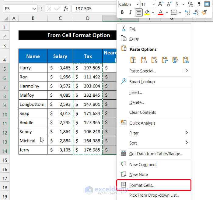
As a result, the Format Cells dialog box will appear.
Then, select the Category as Currency or Accounting. In our case, we kept the Accounting option for better visualization of our dataset.
In the box on the right side of the title Decimal Places, write down 0 on your keyboard. You can also keep clicking the down arrow to reduce the number until 0 appears.
Finally, click OK.

You will see that all values were rounding to their nearest round dollar within a blink.

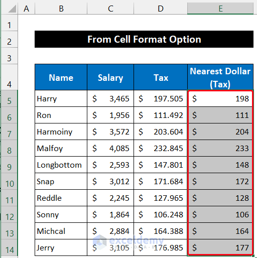
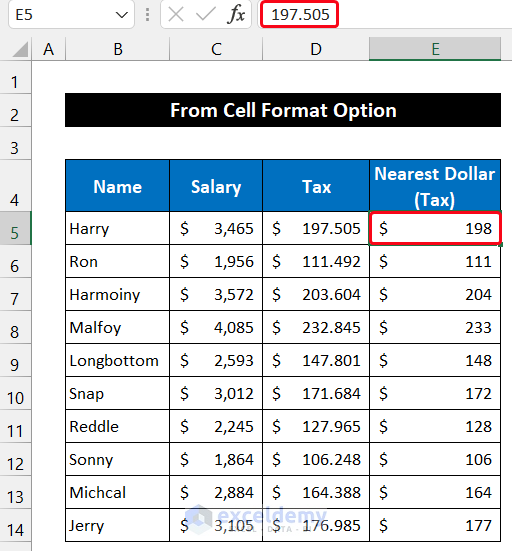
However, if you select any cell in the range E5:E14 and look at the Formula Bar, you can see the original value like column D.

Thus, we can that our rounding method worked successfully and we were rounding the tax payment to the nearest dollar.

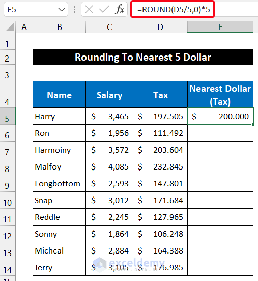
Round up to Nearest 5 Dollar in Excel

According to this process, we will round up the tax payment value to the nearest 5 dollar. This type of rounding is often used in business to provide a consumer with some reduction facility on the payment. We will use the same dataset that we used in our previous method. You have to modify it for your dataset. We will use the ROUND function to get the value. The process is explained below:

📌 Steps:

At first, select cell E5.
Now, write down the following formula into the cell.

=ROUND(D5/5,0)*5

Here, 0 is the num_digits that help us to round up to the decimal.

Press the Enter key.

Then, double-click on the Fill Handle icon to copy the formula up to cell E14.

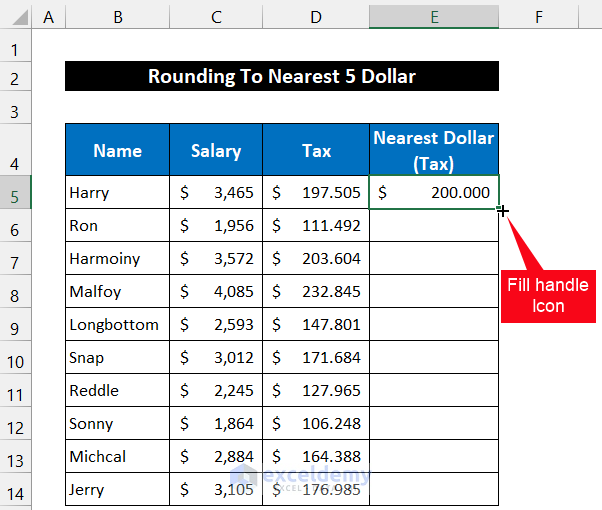
In the end, you will see that all values were rounding to their nearest 5 dollar.

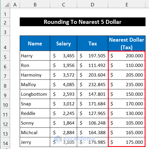
Finally, we can that our formula worked effectively and we are rounding the tax payment to the nearest dollar.

Read More: Round off Formula in Excel Invoice

Download Practice Workbook

Download this practice workbook for practice while you are reading this article.

Rounding to Nearest Dollar.xlsx

Conclusion

That’s the end of this article. I hope that this article will be helpful for you and you can perform the rounding to the nearest dollar in Excel. Please share any further queries or recommendations with us in the comments section below if you have any further questions or recommendations.

Don’t forget to check our website ExcelDemy for several Excel-related problems and solutions. Keep learning new methods and keep growing!

<< Go Back to Rounding in Excel | Number Format | Learn Excel

Get FREE Advanced Excel Exercises with Solutions!

Rounding to Nearest Dollar in Excel (6 Easy Ways)

Rounding to Nearest Dollar in Excel: 6 Easy Ways

1. Using ROUND Function for Rounding to Nearest Dollar

2. Applying MROUND Function

3. Use of ROUNDUP Function

4. Utilizing CEILING Function

5. Rounding to Nearest Dollar Using Decrease Decimal Command

6. Applying Built-in Format Cells Command

Round up to Nearest 5 Dollar in Excel

Conclusion

Related Articles

Leave a reply Cancel reply