How to Merge Rows Based on Criteria in Excel (4 Easy Ways)

Merging rows may sound like quite a complex process in Excel. Especially when it is required based on specific criteria. Therefore, here is a complete solution for you. In this article, we will discuss how to merge rows based on criteria in Excel in 4 easy ways.

How to Merge Rows Based on Criteria in Excel: 4 Easy Ways

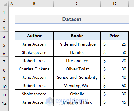
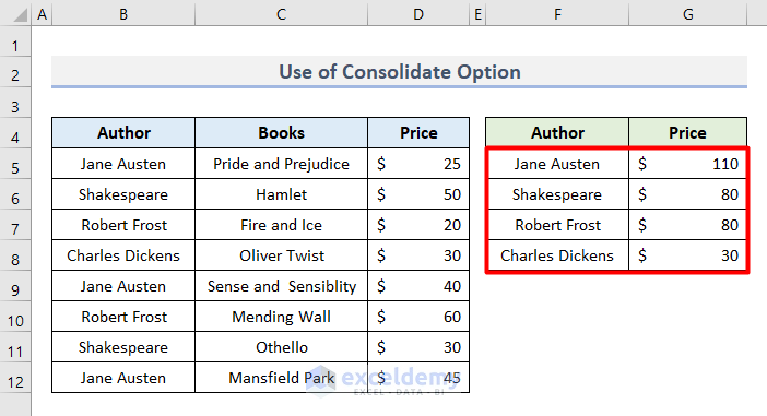
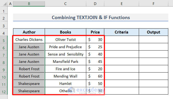
Let’s get into the data table first. Here, I have taken a dataset consisting of 3 columns named Author, Books, Price, and 9 rows. The information is placed in the Cell range B4:D12. Now, let us merge rows where Book names will be combined based on the criteria Author. For this follow the methods below.

1. Use Consolidate Option to Merge Duplicate Values in Excel

In this first method, we will merge rows with the Consolidate option in Excel. Let’s see how the process works.

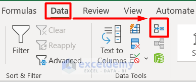
First, select Data > Data Tools > Consolidate.

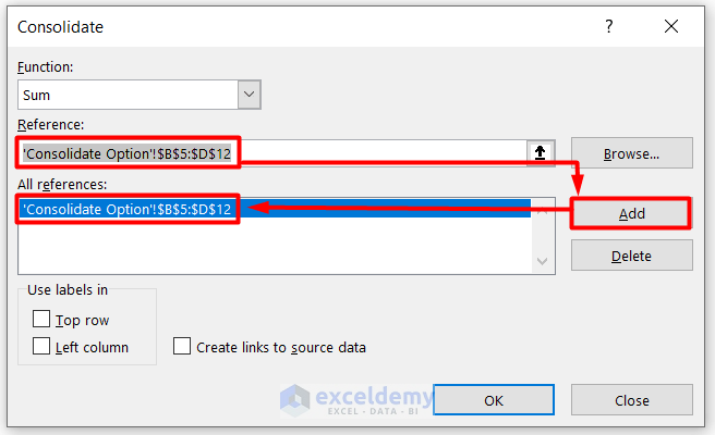
Then, the Consolidate dialog box will appear.
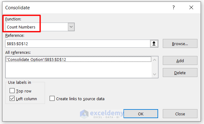
Here, select the whole data range as Reference and then click on Add to insert the range in the All references box.

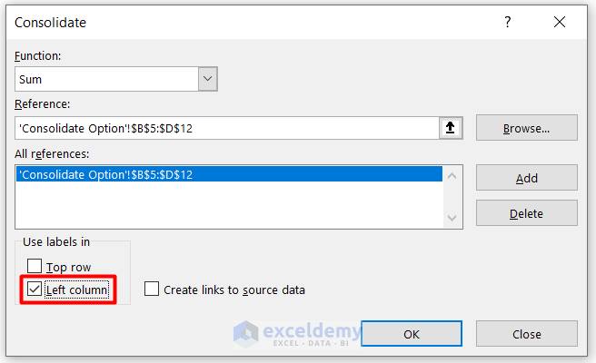
Following this, click on Left Column and press OK.

As a result, the duplicate cells of the Author column will be merged and their respective Price values will be added.

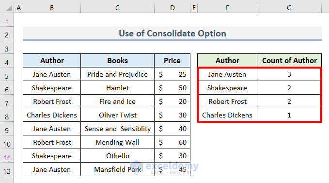
In the above scenario, we have tried to use the SUM function of the Consolidate option. But based on other criteria like counting the number of repetitions of the author names against the merged author name, go through these steps.

For this, select Count Numbers under the Function list in the Consolidate dialogue box as below.

Finally, press OK and the following table will appear.

2. Combine TEXTJOIN & IF Functions to Merge Same Texts Based on Criteria

Another method to merge rows is by combining the TEXTJOIN function and the IF function. To do the task, go through the process below.

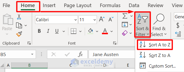
First, select the Author column in the dataset.
Then, choose Home > Editing > Sort & Filter > Sort A to Z.

Following this, select Expand the selection > Sort in the Sort Warning window.

After that, the following sorted data will appear.

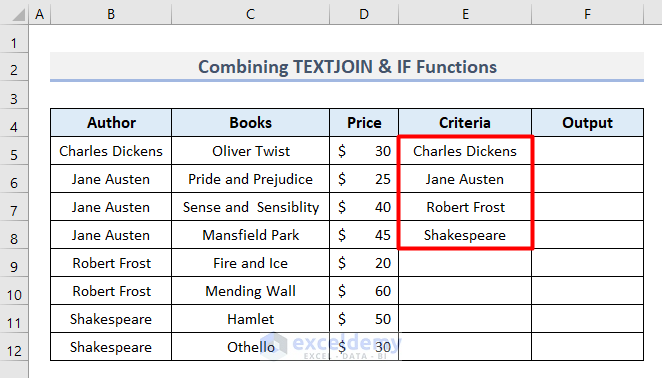
Now, insert the Author names in the Cell range E5:E8 under the Criteria column.

Then, insert this formula in Cell F5.

=TEXTJOIN(", ",TRUE,IF($B$5:$B$12=E5,$C$5:$C$12,""))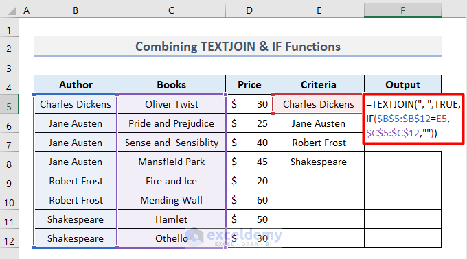

In the formula, the TEXTJOIN function combines the texts from the Cell range C5:C12. Then, the IF function states the condition where $B$5:$B$12=E5 and the TRUE function determines that the condition is true.

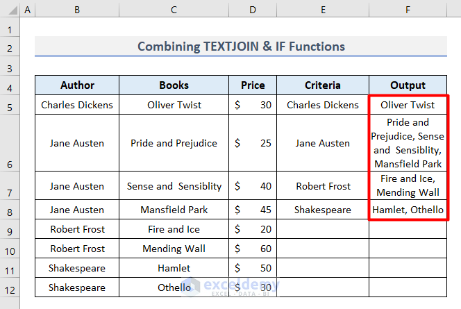
Lastly, press Enter > Autofill.
That’s it, you will get the merged rows of book names.

Read More: Excel Merge Rows with Same Value

3. Use Pivot Table to Merge Rows Based on Criteria

In this section, to merge rows on the basis of the same authors and then with respect to their name the sum of the price of their book the Pivot Table option will be used. Let’s see how it works.

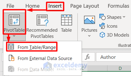
First, select Insert > Pivot Table > From Table/Range.

Next, the PivotTable from table or range dialog box will appear.
Here, you will notice the selected range is visible in the Table/Range box.
Along with it, choose New Worksheet as the location for Pivot Table.

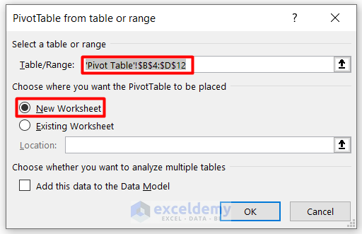
Then, press OK and you will be directed to a new worksheet.
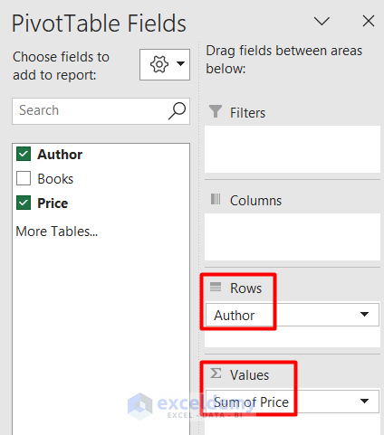
Now, drag Author to the Rows field and Price to the Values.

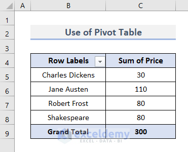
Finally, the following table will appear where the same rows will be merged in the Author column, and with respect to the authors, the prices are added up.

4. Insert COUNTIF Function to Merge Rows in Excel

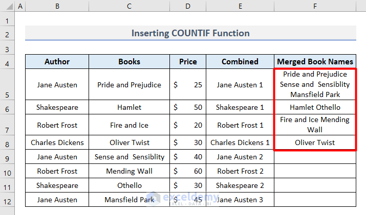
In this section, we will join all of the Books with respect to each Author. For this, follow the process described below.

First, insert this formula in Cell E5.

=B5&" "&COUNTIF($B$5:$B5,B5)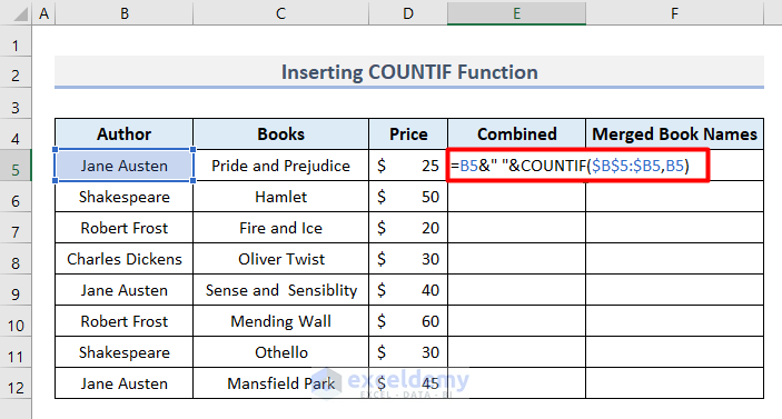

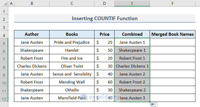
Here, the COUNTIF function counts cells based on the condition given in Cell B5.

Then, drag it all the way to the Combined column the following result will appear.

After that, you have to use the following logical function in Cell F5.

=IF($B5&" "&1=E5, INDEX(C4:C12,MATCH($B5&" "&1,E4:E12,0))&" "&IFERROR(INDEX(C4:C12,MATCH($B5&" "&2,E4:E12,0)),"")&" "&IFERROR(INDEX(C4:C12,MATCH($B5&" "&3,E4:E12,0)),"")&" "&IFERROR(INDEX(C4:C12,MATCH($B5&" "&4,E4:E12,0)),""),"")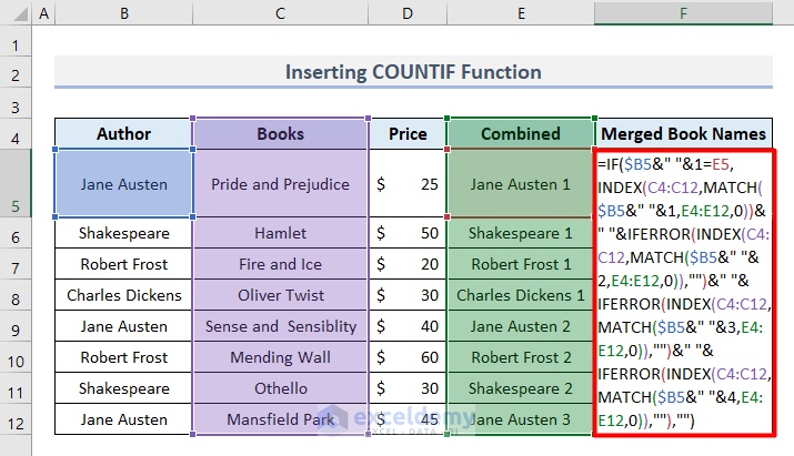

🔎 How Does the Formula Work?

$B5&” “&1=E5: Here, this part states the condition where B5=E5.
IFERROR(INDEX(C4:C12,MATCH($B5&” “&2,E4:E12,0)): The INDEX function returns the value of B5 among Cell range C4:C12 and the MATCH function matches it with the range E4:E12. Along with it, type 0 for an exact match. Lastly, the IFERROR function finds and omits any possibility of error occurrence. This part of the formula is used 3 times because we found Jane Austen 3 times in the criteria of Author.
&” “&: The Ampersand (&) and Quotation Marks (“ “) with a Space help to create spaces between each text.

Now, press Enter to see the first value of merged rows.

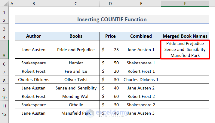
Lastly, use the Autofill command to get all the Merged Book Names as follows.

Download Practice Workbook

Get this practice file and try the process by yourself.

Merge Rows Based on Criteria.xlsx

Conclusion

Hope that this article will help you how to merge rows based on criteria in Excel. We tried to show you it in possible 4 easy ways. Feel free to comment if anything seems difficult to understand.