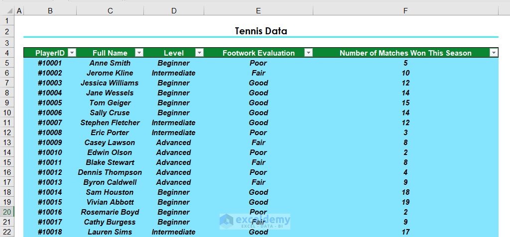
How to Make Excel Tables Look Good (8 Effective Tips)

Excel Tables are extremely useful for organizing and showcasing data. They can also be formatted using the features available in Excel, in order to be visually striking and appealing. We are going to look at some handy tips to make Tables in Excel look great.

So, let’s get started with a simple example to illustrate how to create a table in Excel and then how to format this Table, using some formatting features and tricks.

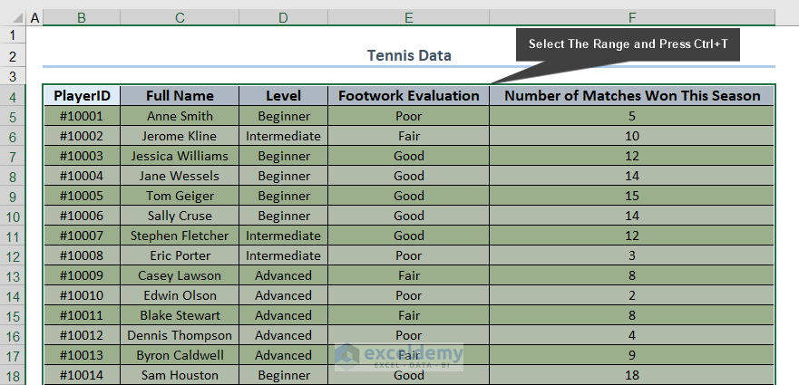
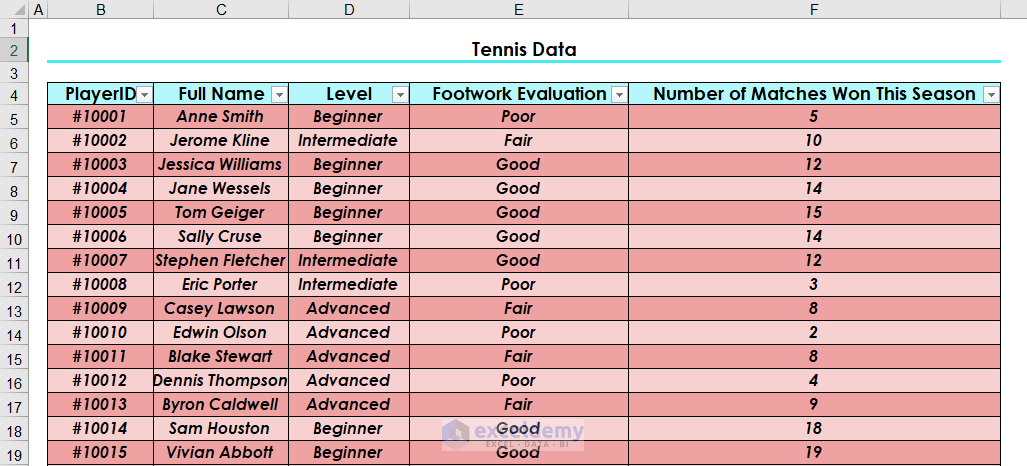
How to Create an Excel Table?

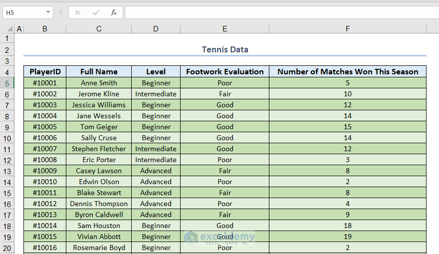
Let’s first have a brief idea of creating an Excel table. After that, we will see how to get Excel tables in a good or professional look.

Apply the following steps to create a table in Excel.

Steps:

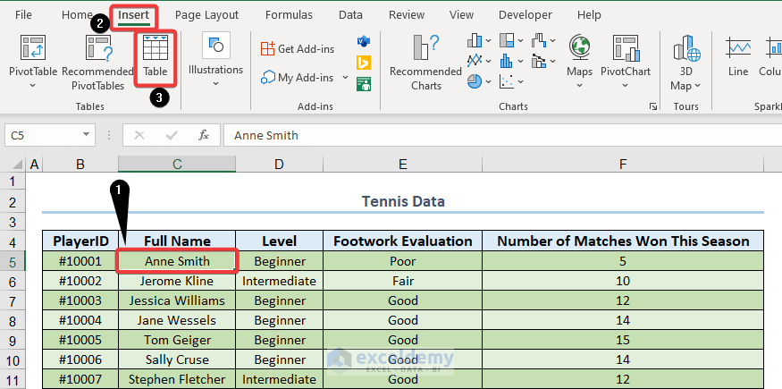
Select a cell from the data set.

The Table option is found on the Insert tab, in the Tables group.

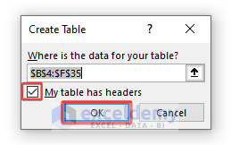
Excel will automatically pick data for you. Check the box next to ‘My table contains headers‘, then click OK.

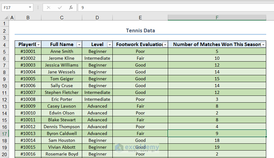
Excel will format a lovely table for you. This may still appear to be a standard data range to you. However, numerous sophisticated capabilities are now available with the press of a button.

Or,

Choose your desired dataset and click the button CTRL+T.

How to Make Excel Table Look Good/Professional

There can be many ways to make Excel tables with an extraordinary look. In this article, we will discuss 8 basic ways to do it.

1. Using Built-In Table Styles to Make Good-Looking Excel Table

You can quickly change the appearance of your newly created Excel Table, using the built-in Table styles in the following way.

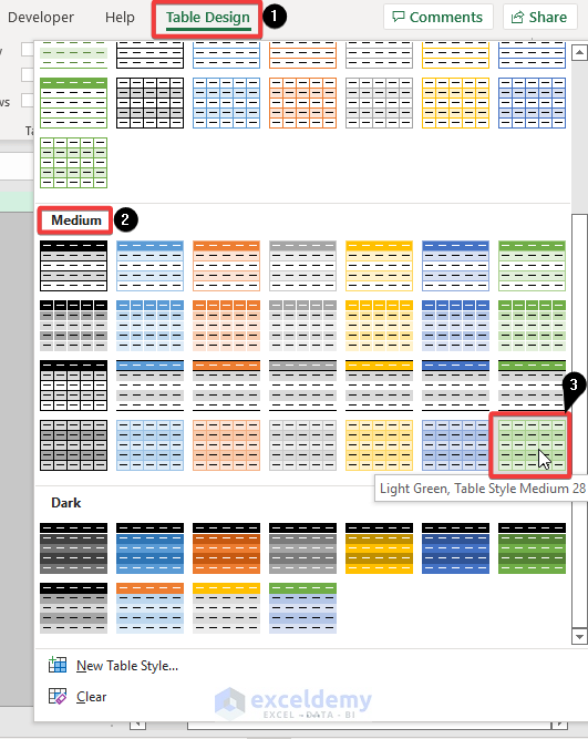
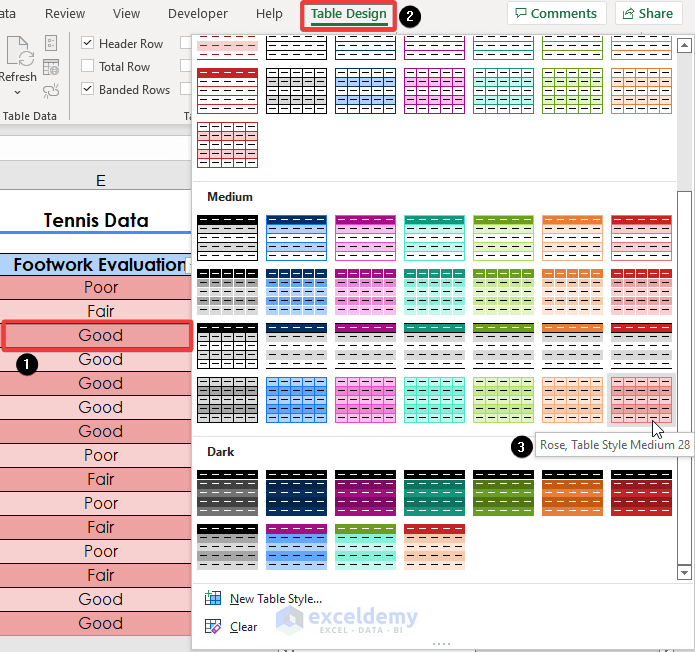
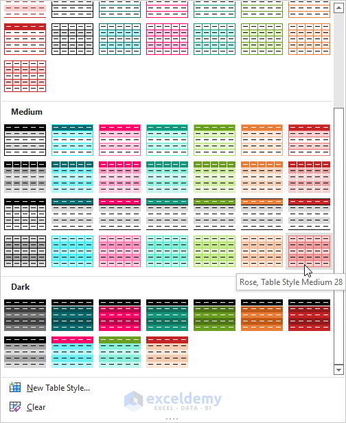
Select any cell in the Footwork table.
Then go to Table Design → Table Styles and click on the drop-down arrow.
Now, choose one of the built-in Table Styles available.
You can get a preview by just hovering over each style.

In this case, we have selected Table Style Medium 28 as shown below.

After applying this style, we get the following table.

The colors used in the Table are drawn from the default Office theme.

2. Changing Workbook Theme Looks Better

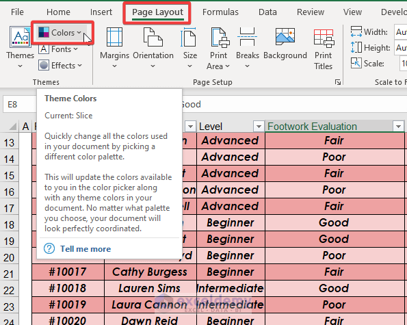
The colors provided in the Table Styles options are drawn from the default Office theme. In order to quickly change the options provided there, one can change the theme of the Workbook.

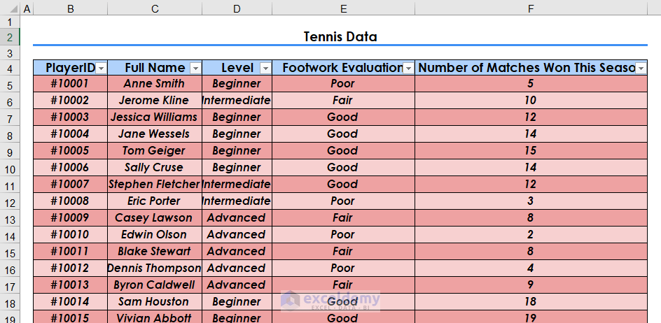
Go to Page Layout → Themes → and click on the drop-down arrow below Themes and select another theme, that is not the default Office theme, in this case, the Slice theme.

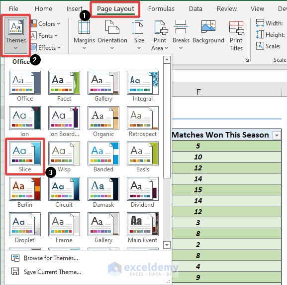
The Table Style draws its colors from the Slice theme and the effect of the change on the actual Excel Table is shown below.

To see the change that has been affected on all the Table Styles options, through changing the theme from Office to Slice, select one cell in the table and go to Table Tools → Design → Table Styles → click on the drop-down arrow, in order to see the alternate color schemes drawn from the new theme.

3. Editing Themes Color Make Excel Table Look Good

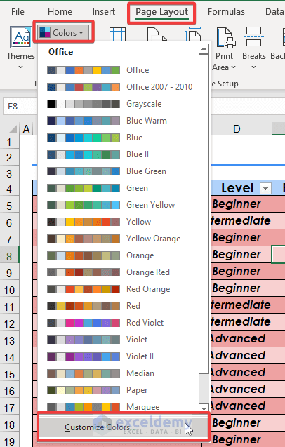
You can also alternatively, change the theme colors yourself, or set the theme colors yourself in order to effect changes in the Table Styles options.

With any theme currently selected, go to Page Layout → Themes → and click on the drop-down next to Colors.

Choose the Customize Colors option.

In the Create New Theme Colors Dialog Box, select the drop-down arrow next to Text/Background – Dark 2 and choose More Colors.

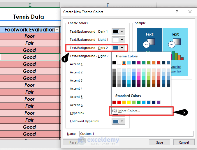
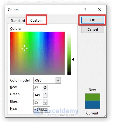
Select the Custom Tab and enter the following values R 87, G 149, and B 35, in order to set this dark green color and click OK.

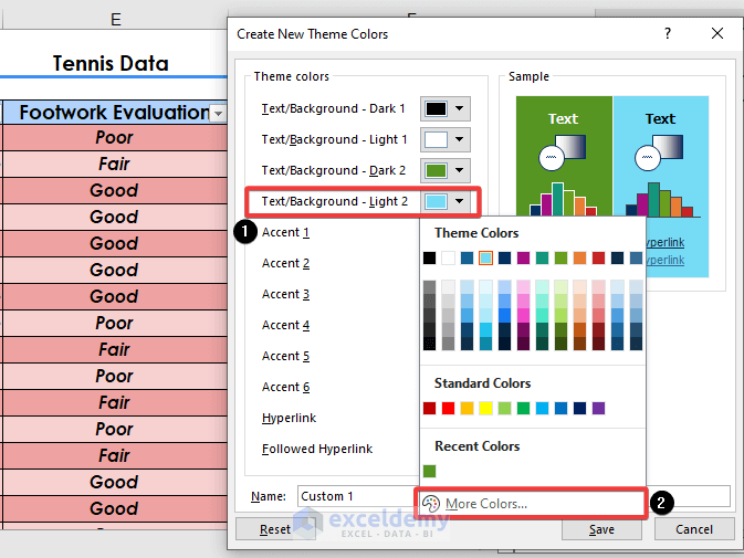
In the Create New Theme Colors Dialog Box, select the drop-down next to Text/Background – Light 2 and choose More Colors.

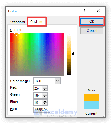
Select the Custom Tab and enter the following values R 254, G 184, and B 10, in order to set this orange color and click OK.

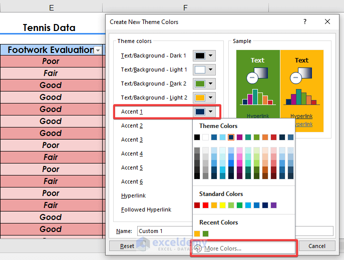
In the Create New Theme Colors Dialog Box, select the drop-down next to Accent 1 and choose More Colors.

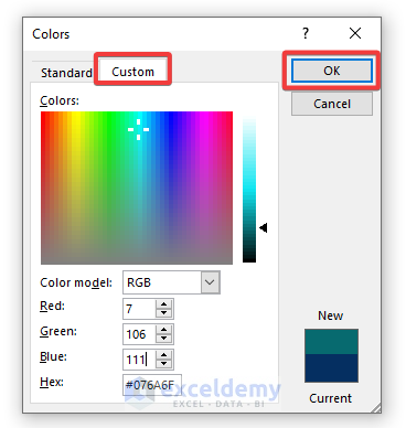
Select the Custom Tab and enter the following values R 7, G 106, and B 111, in order to set this dark turquoise color and click OK.

Now, in the Create New Theme Colors Dialog Box, select the drop-down next to Accent 2 and choose More Colors.

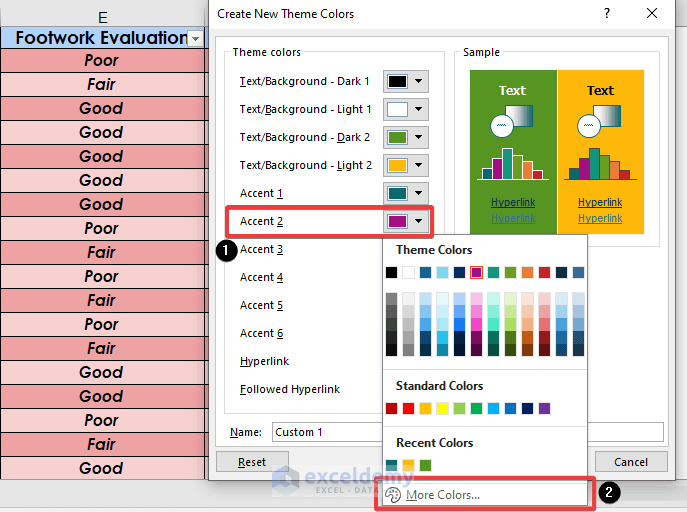
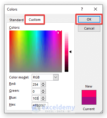
Select the Custom Tab and enter the following values R 254, G 0, and B 103, in order to set this pink color and click OK.

Give your new customized theme color, set a name, and click Save.

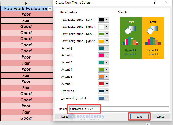
The effect of changing the theme colors to this customized set is immediately reflected in the Footwork Table, as shown below.

It is also reflected in the Table Styles Options, going to Table Tools → Design → Table Styles and clicking on the drop-down arrow, in order to see the new Table Styles drawn from the new customized theme colors set.

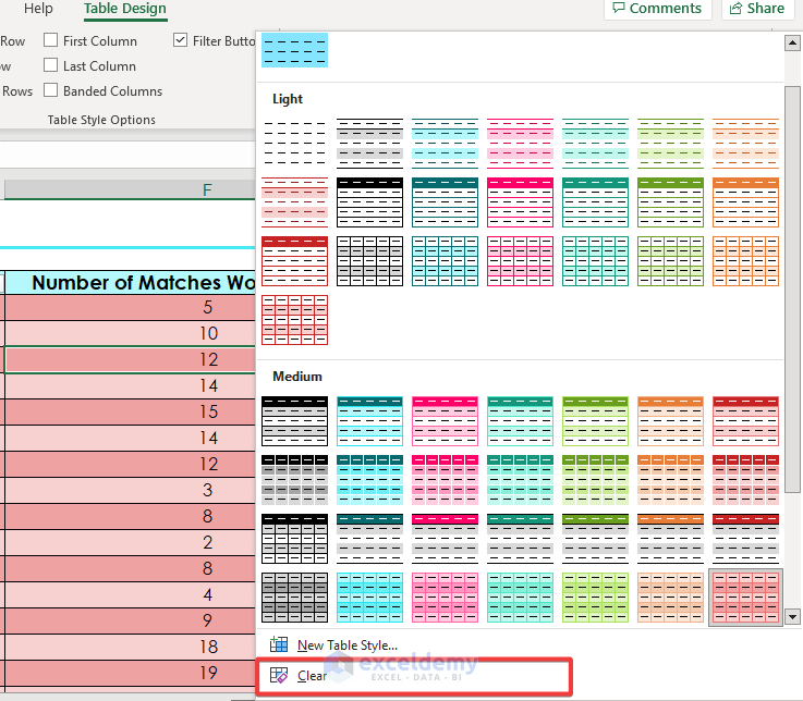
4. Clearing Style from an Excel Table

You can also totally clear the style from a Table, by selecting one cell in the Table going to Table Tools → Design → Table Styles, and clicking on the drop-down arrow next to Table Styles.

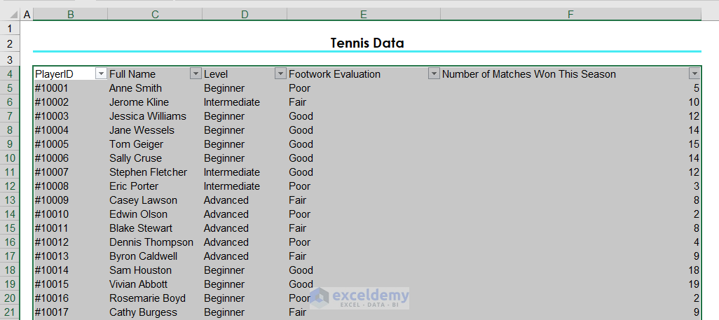
Select Clear in order to remove table the formatting associated with the specific table style chosen.

Any formatting associated with the specific table style chosen is now cleared as shown below.

5. Creating Custom Excel Table Style for Good-Looking

You can create your own Table Style in Excel and format the header row, columns in the Table, and rows in the Table precisely.

With a cell in the Table selected, go to Table Tools → Design → Table Styles, click on the drop-down arrow next to Table Styles, and select New Table Style.

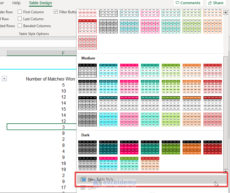
One can now format individual elements of the Table, using the New Table Style Dialog Box.

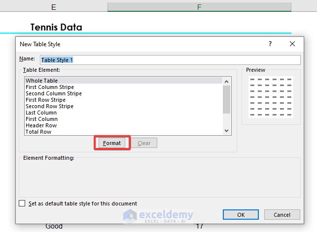
The first element we are going to format is the Whole Table element. Select the Whole Table and then choose Format.
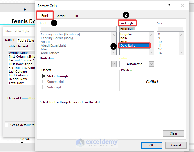
The Format Cells Dialog Box should appear, choose the Font Tab, and under font style choose Bold Italic.

Go to the Fill Tab, under the Background Color option, choose More Colors.

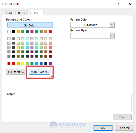
Select the Custom Tab, set R 133, G 229, and B 255 as shown below, and then click OK.

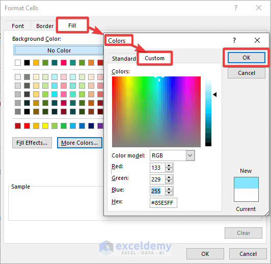
Click OK again.
Now select the Header Row element as shown below and click Format.

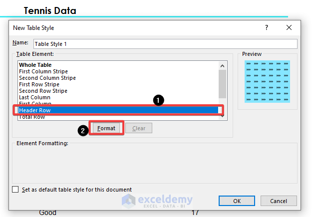
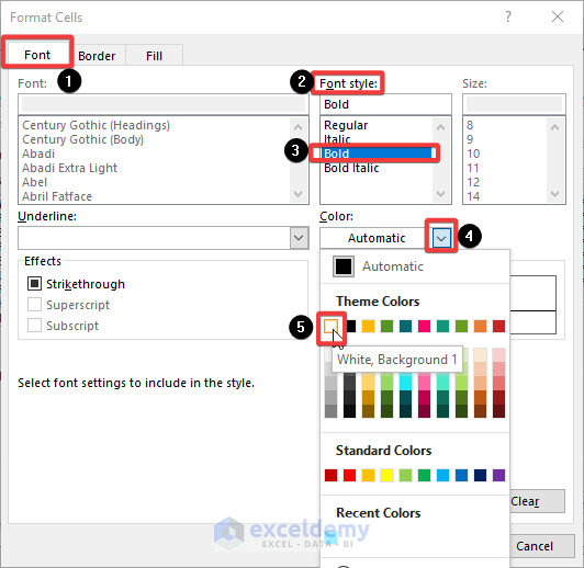
The Format Cells Dialog Box should appear as before, choose the Font Tab, and under Font Style choose Bold and change the font color to White, Background 1.

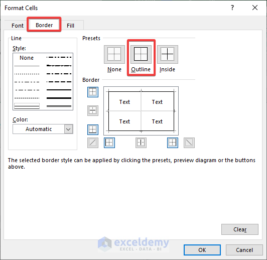
Choose the Border Tab, select the thick line style, and the color Gray – 25%, Background 2, Darker 50%.

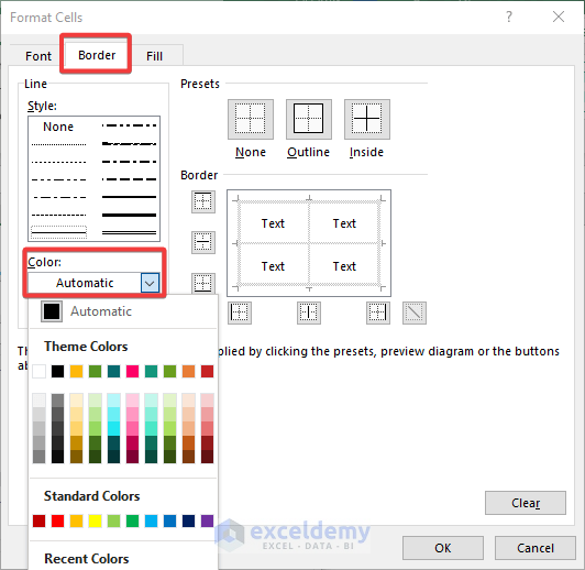
Choose Outline, in order to outline the entire Header Row with this border formatting.

Then select the Fill Tab, under Background Color, choose More Colors.

Select the Custom Tab, set R 11, G 135, and B 52 as shown below, and then click OK.

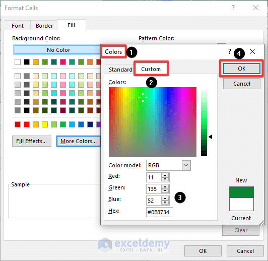
Click OK again.
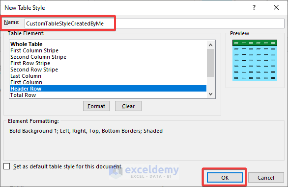
Give your new Table Style a name and check the Set as default table style for this document option, in order to ensure that all tables created in the workbook have this format, in order to contribute to a streamlined look.

Applying this Custom Table Style to the Footwork Table results in the following look.

Read More: Navigating Excel Table

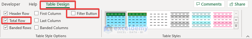
6. Adding Total Row and Turn the Filter Button Off

One can also add a Total Row and turn the filter buttons of the Table off, quite easily.

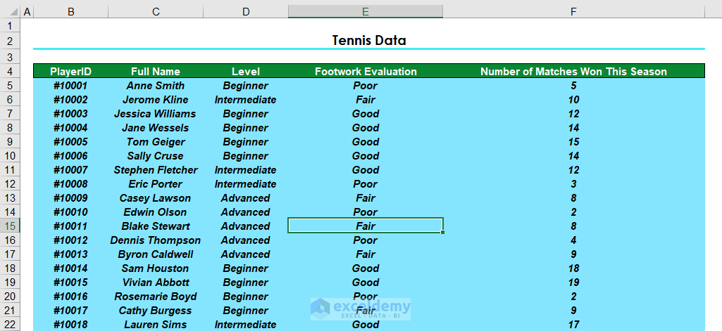
With one cell in your table selected, go to Table Tools → Design → Table Style Options and check Total Row in order to add a Total Row, and uncheck the Filter Button in order to turn off the filter buttons of the header row as shown below.

As a result, the table will have the following look.

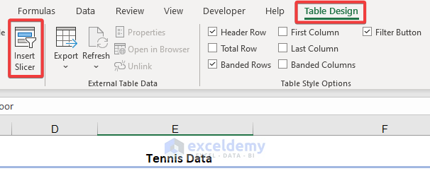
7. Inserting Slicers to Make Excel Table Looks Good

Table Slicers allow one to filter the data in the Table according to the column categories, these slicers can also be formatted to match the overall Table formatting.

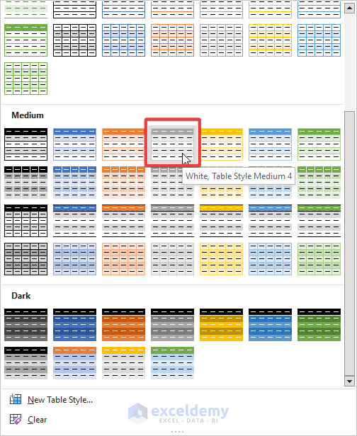
First things first, format the Table with a certain style, by going to Table Tools → Design → Table Styles and choosing Table Style Medium 4 (make sure the theme is the default Office theme).

Now the entire table has the format with this style as shown below.

With one cell in the table selected, go to Table Tools → Design → Tools → Insert Slicer.

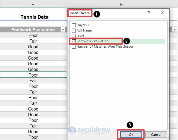
Choose one or more slicers to filter the data by, in this case, we’ll choose Footwork Evaluation as shown below and then click OK.

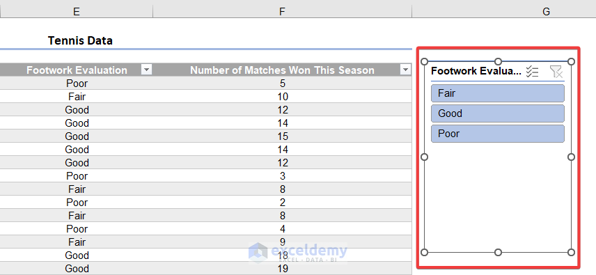
The Slicer with the default style appears as shown below.

One can change the style of the slicer using one of the built-in styles. With the slicer selected, go to Slicer Tools → Options → Slicer Styles, select one of the default built-in Styles, and choose Slicer Style Light 2 as shown below.

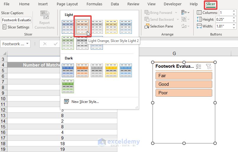
This changes the Slicer Style to the following format.
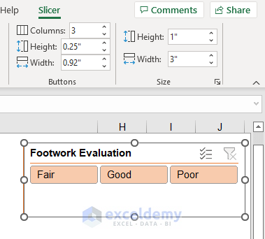
With the Slicer selected, go to Slicer Tools → Options → Buttons and Change the number of columns to 3, and then with the Slicer still selected, go to Slicer Tools → Options → Size and Change the height of the slicer to 1 inch and the width to 3 inches as shown below.

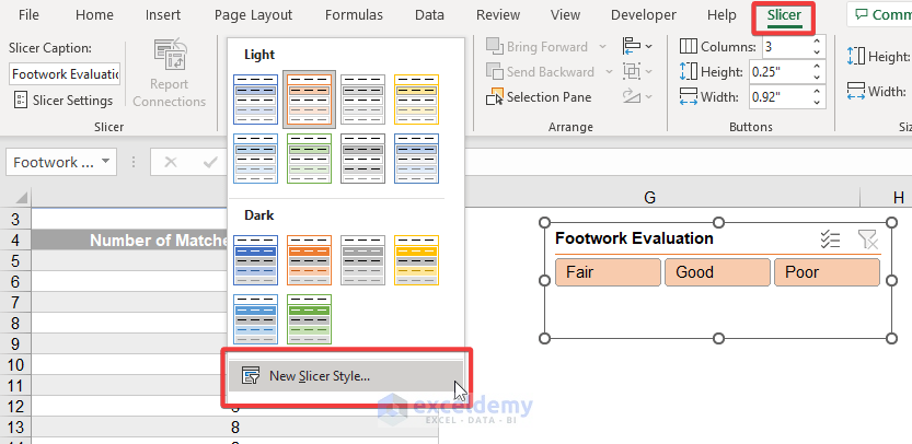
With the slicer still selected, we now want to create a new custom Slicer Style to match the Table Style we chose. So, we go to Slicer Tools → Options → Slicer Styles, we click on the drop-down next to Slicer Styles, and select New Slicer Style as shown below.

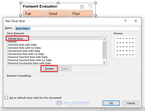
In the New Slicer Style Dialog Box, choose the Whole Slicer element and then click Format.

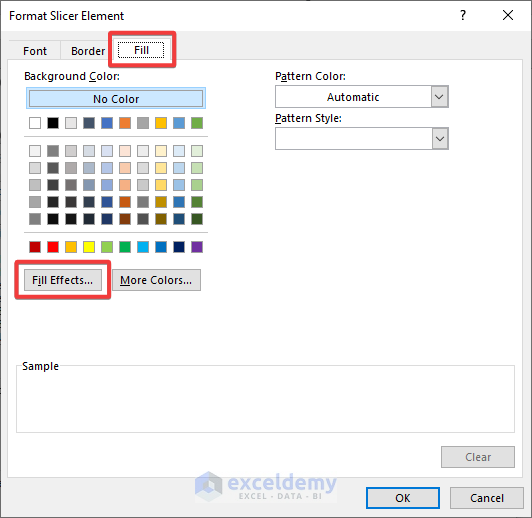
In the Fill Tab, under Background Color, choose Fill Effects.

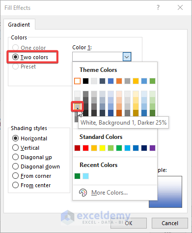
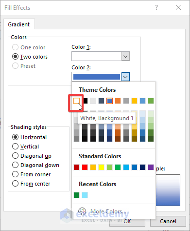
Using the Fill Effects Dialog Box, change Color 1 to White, Background 1, Darker 25%, and change Color 2 to White, Background 1 as shown below.

Similarly, add more colors.

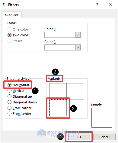
Under Shading styles make sure Horizontal is selected and choose the third variant as shown below.

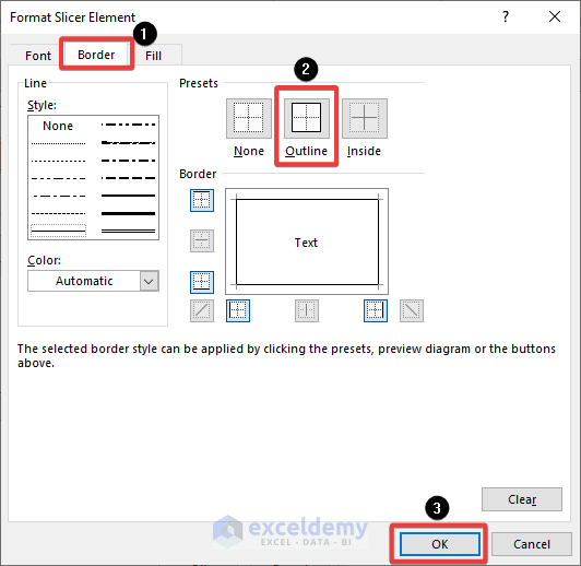
Click OK and then select the Border Tab, choose the thin line style and White Background 1, Darker 35%, and then select Outline as shown below.

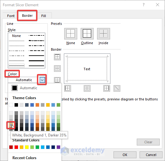
Choose a proper outline.

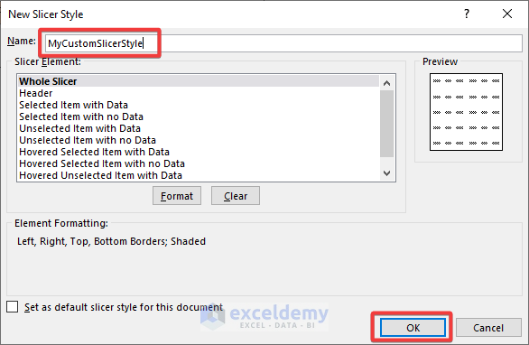
Click OK and then name your newly created Slicer Style as shown below and click OK.

Apply the new Slicer Style you just created.
Go to View → Show → and uncheck Gridlines in order to see the full effect of the formatting.

8. Converting a Table Back to a Range

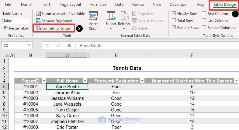
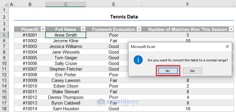
In order to convert a Table back to a range, select a cell in the Table as shown below and go to Table Tools → Design → Tools → Convert to Range.

A Dialog Box should appear asking you if you want to convert the Table to a normal range, select Yes.

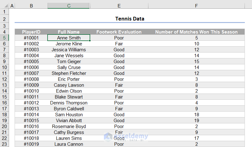
The Table should now be converted to a normal range but with the formatting selected still intact as shown below.

Download Practice Workbook

You can download the following practice workbook, where we have placed the formatted table and original table in separate worksheets.

Making Excel Tables Look Good.xlsx

Conclusion

You can create and format tables extensively in Excel, it is often necessary to format tables and a professional look for visual appeal or printing purposes. Please feel free to comment and tell us about your Table formatting tricks and tips for Excel.