You may be working with a large amount of data in Microsoft Excel which contains duplicated data. You might want to highlight the duplicates but keep one, which is an easy and time-saving task. Excel has some easy and useful ways to highlight duplicates but keep one. Today, in this article, we’ll learn four quick and suitable ways to highlight duplicates in Excel but keep one effectively with appropriate illustrations.
How to Highlight Duplicates in Excel but Keep One: 4 Suitable Ways
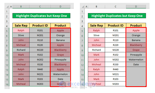
Let’s assume we have an Excel large worksheet that contains the information about several sales representatives of Armani Group. The name of the Products and the Products ID is given in Columns D, and C respectively. We will highlight duplicates but keep one in Excel using the Conditional Formatting Command, The COUNTIF function, and so on. Here’s an overview of the dataset for today’s task.
1. Use Conditional Formatting Command to Highlight Duplicates but Keep One in Excel
Here, we will use conditional formatting to highlight duplicates but keep one in Excel. We will do that easily from our dataset. From our dataset, we will highlight the duplicates of the name of sales representatives but keep one. Let’s follow the instructions below to highlight duplicates but keep one!
Step 1:
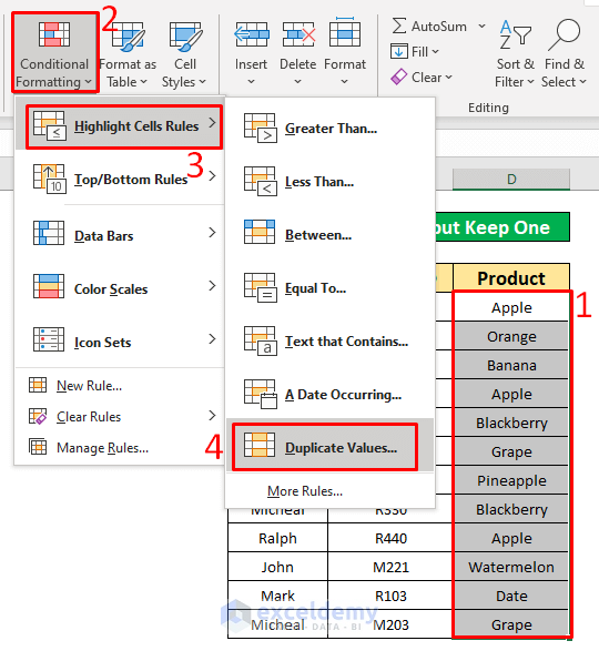
- First of all, select cells that we want to highlight duplicates but keep one. From our dataset, we select cells from B5 to B16. Then, from your Home tab, go to,
Home → Styles → Conditional Formatting → Highlight Cells Rules → Duplicate Values
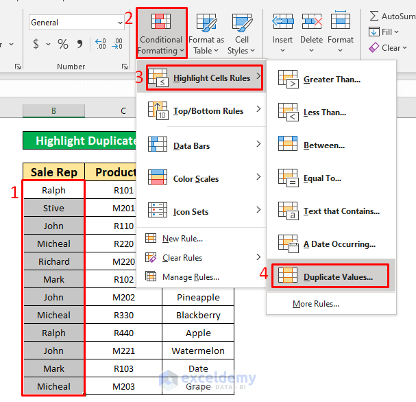
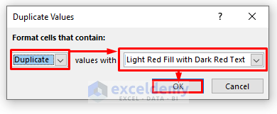
- Hence, a dialog box named Duplicate Values pops up. From the Duplicate Values dialog box, firstly, select the Duplicate values with Light Red Fill with Dark Red Text option from the Format cells that contain Secondly, press OK.
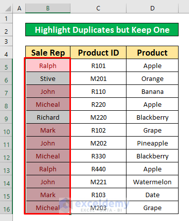
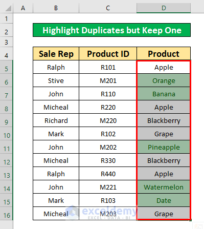
- After pressing OK, you will be able to highlight the duplicates value that has been given in the below screenshot.
Step 2:
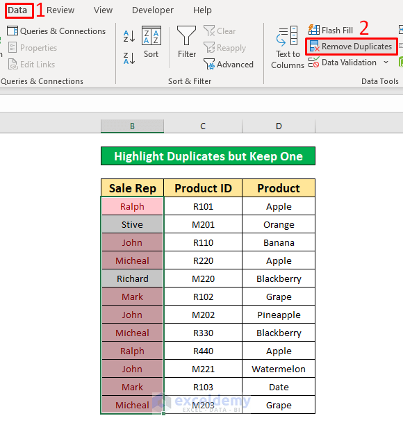
- Now, we will keep one duplicate. To do that, from your Data tab, go to,
Data → Data Tools → Remove Duplicates
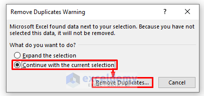
- Further, a warning dialog box named Remove Duplicates Warning will appear in front of you. From that warning box, firstly, select Continue with the current selection. Secondly, press Remove Duplicates.
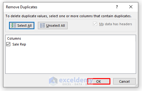
- As a result, a Remove Duplicates window pops up. From that window, press OK.
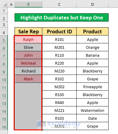
- After completing the above process, you will be able to highlight duplicates but keep one that has been given in the below screenshot.
Read More: How to Highlight Duplicates in Two Columns Using Excel Formula
2. Highlight Duplicates or Unique Values Using Conditional Formatting in Excel
Now, we’ll highlight duplicates or unique values by applying the conditional formatting command. This is an easy and time-saving task. From our dataset, we will highlight the unique products. Let’s follow the instructions below to learn!
Steps:
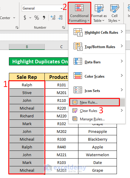
- First, select cells from B5 to B16. Then, from your Home tab, goto,
Home → Styles → Conditional Formatting → Highlight Cells Rules → Duplicate Values
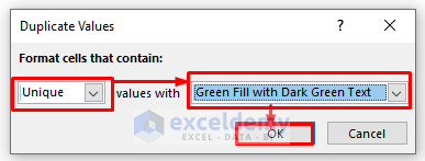
- Further, a dialog box named Duplicate Values will appear in front of you. From the Duplicate Values dialog box, firstly, select the Unique values with Green Fill with Dark Green Text from the drop-down box. Secondly, press OK.
- While pressing OK, you will be able to highlight the unique values that have been given in the below screenshot.
3. Highlight Duplicates but Keep One Based on Occurrence Using New Rule of Conditional Formatting
However, you can also highlight duplicates based on the time of occurrences. We will be seeing the occurrences without the 1st one, only the second one or 3rd time. In addition, I would like to mention by observing the results for the 3 types you can easily learn to modify the formula to get other occurrence-based results. Let us divide the 3 types and see them one by one.
3.1 Duplicates without First Occurrence
Follow the steps to highlight duplicates without the first occurrence.
Steps:
- First, select cells from B5 to B16. Then, from your Home tab, go to,
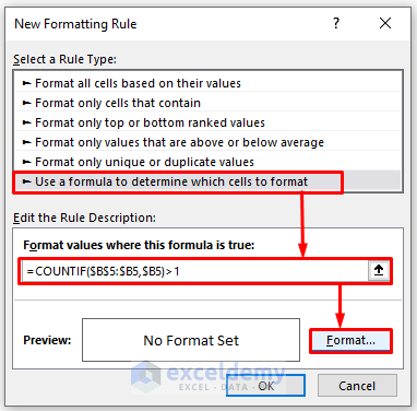
Home → Styles → Conditional Formatting → New Rule
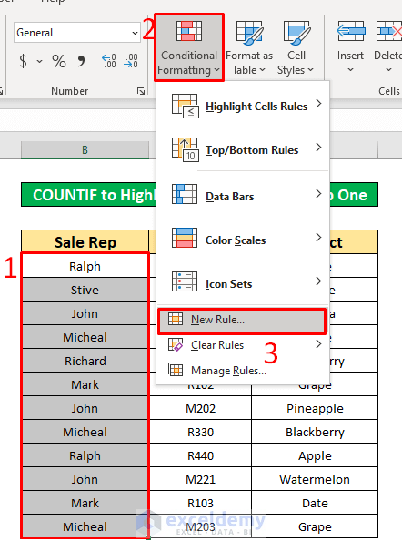
- A dialog box named New formatting Rule will appear. Follow the steps for the New formatting Rule dialog box. Firstly, select Use a formula to determine which cells to format from the Select a Rule Type: Secondly, write the below formula in the Format values where this formula is true:. The COUNTIF function is,
=COUNTIF($B$5:$B5,$B5)>1- Hence, press the Format option.
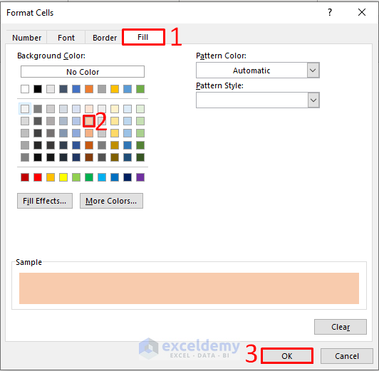
- After clicking on the Format option, a Format Cells dialog box pops up. From that dialog box, firstly, select the Fill Secondly, select any color from the Background Color menu. We have chosen light golden color. At last, click OK.
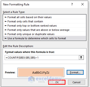
- Hence, you will go back to the New formatting Rule dialog box. Finally, you have to click OK.
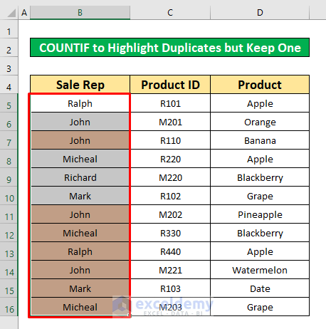
- While completing the above process, you will be able to highlight duplicates without the first occurrence that has been given in the below screenshot.
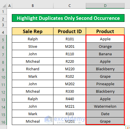
3.2 Second Occurrence of Duplicates Only
For highlighting the data only 2nd time in the dataset you can follow the steps below.
Steps:
- First of all, select cells D5 to D16.
- After that, perform similarly according to sub-method 3.1 except the formula which is applied in the Format values where this formula is true: Now, type the below formula in that type box. The formula is,
=COUNTIF($B$5:$B5,$B5)=2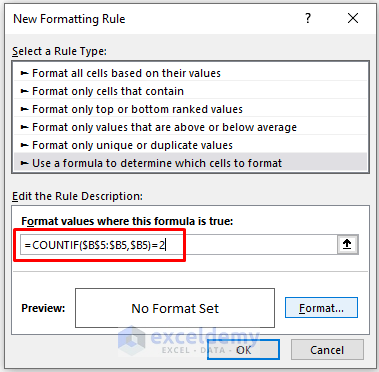
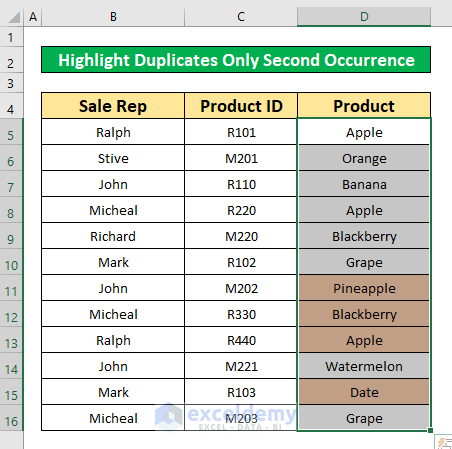
- After repeating the sub-method, you will get your desired output which has been given in the below screenshot.
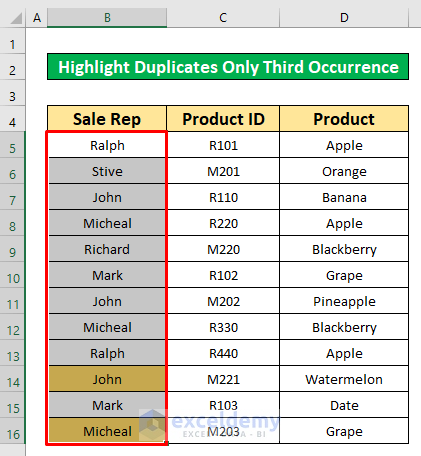
3.3 Values Occurring Third Time
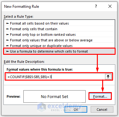
To highlight the third occurrence and above we have to follow the steps which are similar to the above two. The only difference is the formula here. For your ease, the instructions are as follows:
Steps:
- First, select cells from B5 to B16. Then, from your Home tab, go to,
Home → Styles → Conditional Formatting → New Rule
- A dialog box named New formatting Rule will appear. Follow the steps for the New formatting Rule dialog box. Firstly, select Use a formula to determine which cells to format from the Select a Rule Type: Secondly, write the below formula in the Format values where this formula is true:. The formula is,
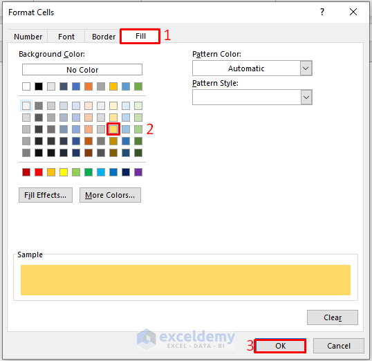
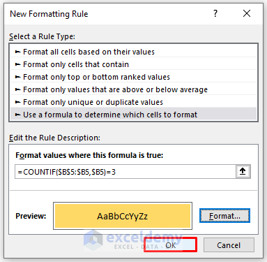
=COUNTIF($B$5:$B5,$B5)=3- Hence, press the Format option.
- After clicking on the Format option, a Format Cells dialog box pops up. From that dialog box, firstly, select the Fill Secondly, select any color from the Background Color menu. We have chosen light golden color. At last, click OK.
- Hence, you will go back to the New formatting Rule dialog box. Finally, you have to click OK.
- After completing the above process, you will be able to highlight duplicates without the third occurrence that has been given in the below screenshot.
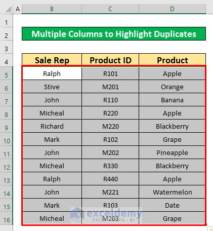
4. Multiple Columns to Highlight Duplicates but Keep One in Excel
Moving forward to duplicates in multiple columns. To highlight duplicates in multiple columns you can use sub-method 3.1. However, you can do this using formula also. Let’s follow the instructions below to learn!
Steps:
- First of all, select cells B5 to D16.
- After that, perform similarly according to sub-method 3.1 except the formula which is applied in the Format values where this formula is true: Now, type the below formula in that type box. The formula is,
=COUNTIF(B$5:$B$14,B5)+COUNTIF(C$5:C5,C5)>1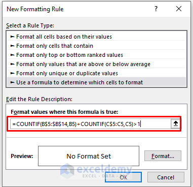
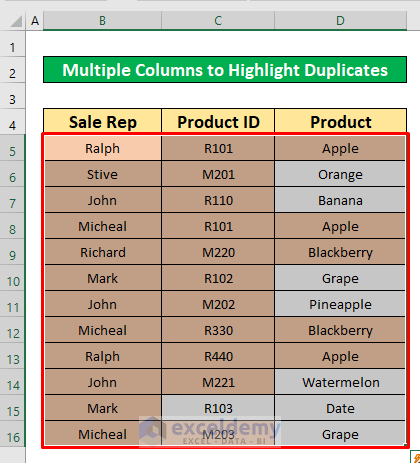
- After repeating the sub-method, you will get your desired output which has been given in the below screenshot.
Read More: How to Highlight Duplicates in Multiple Columns in Excel
Things to Remember
👉 To acquire the desired outcome, you must carefully follow all of the procedures and make any required adjustments to the cell references.
Download Practice Workbook
Download this practice workbook to exercise while you are reading this article.
Conclusion
I hope all of the suitable methods mentioned above highlight duplicates but keeping one will now provoke you to apply them in your Excel spreadsheets with more productivity. You are most welcome to feel free to comment if you have any questions or queries.
Related Articles
- Highlight Cells If There Are More Than 3 Duplicates in Excel
- How to Highlight Duplicates in Excel with Different Colors
- How to Highlight Duplicates in Two Columns in Excel
- How to Highlight Duplicate Rows in Excel
- Highlight Duplicates across Multiple Worksheets in Excel
- [Fix:] Highlight Duplicates in Excel Not Working
<< Go Back to Highlight Duplicates in Excel | Duplicates in Excel | Learn Excel
Get FREE Advanced Excel Exercises with Solutions!
