On the off chance that there is data on our worksheet we don’t have to see, we can hide those that we would rather not see. Then, when we want that information, we can disclose it by following a few strategies. In this article, we will learn how to unhide rows in Excel.
How to Unhide Rows in Excel: 8 Quick Ways
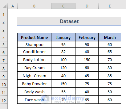
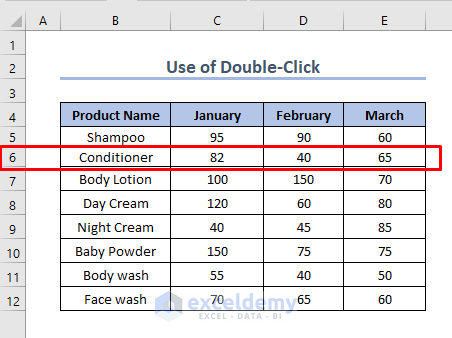
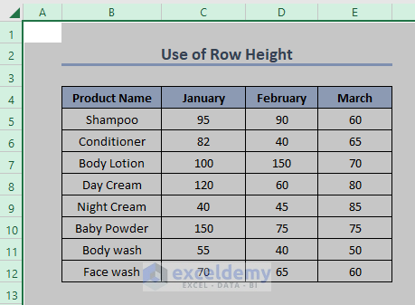
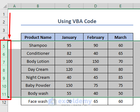
We will utilize this basic dataset which contains some item names and the complete sell information in the long stretch of January to March.
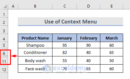
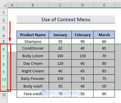
1. Show Hidden Rows Using Context Menu in Excel
Generally, It’s quite easy to spot the hidden rows in a spreadsheet. The way to find them is to look for a double line among the rows heading. Let’s go through the following steps to see how this feature works to unhide rows in Excel.
Steps:
➣To begin, choose the rows that you want to reveal. It’s as simple as picking one row above and one row below the row or rows you want to see. The Unhide option can be found by right-clicking on the mouse.

➣This makes the hidden rows unhide again. The rows are then shown on the spreadsheet.
2. Unhide Rows by Double Clicking
In many cases, the quickest way to reveal the hidden rows is by double-clicking. The beauty of this strategy is that it eliminates the necessity for selection.
Steps:
➣Simply move the mouse over the hidden rows headings and double-click until the mouse pointer becomes a split two-headed arrow.
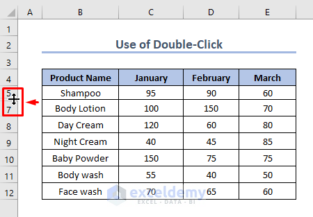
➣The rows now appear in the workbook.
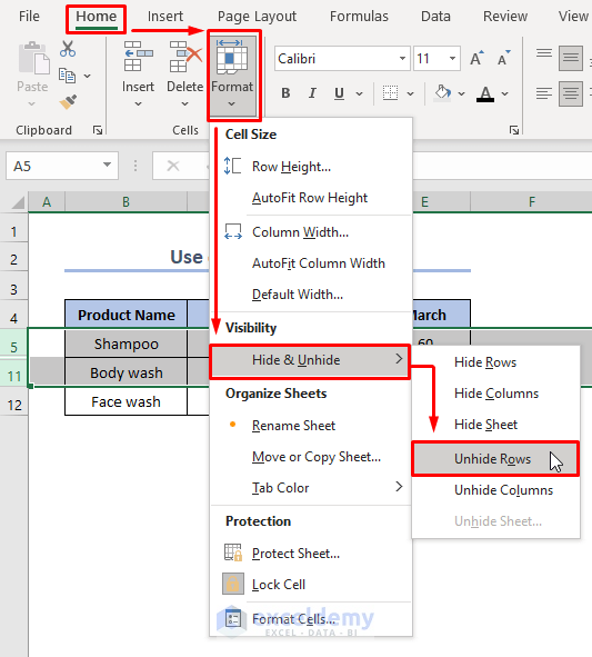
3. Excel Unhide Rows with Format Feature
Similar to the above dataset, we can also unhide rows from the Format feature in the ribbon.
Steps:
➣We’ll choose the rows we wish to unhide again in the same way we did before. To Unhide rows, go to the Home tab > Cells section > select Format > then Hide & Unhide from the menu. Then, click Unhide Rows.
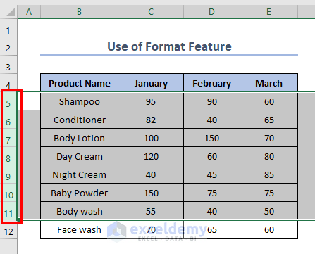
➣Finally, the hidden rows are visible again.
Read More: [Fixed!] Excel Rows Not Showing but Not Hidden
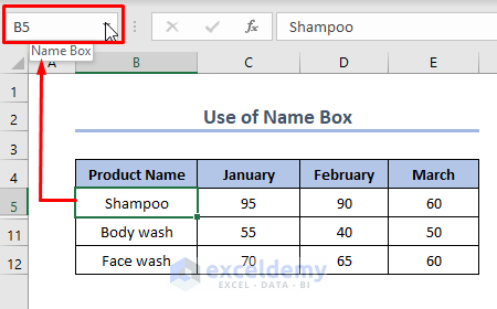
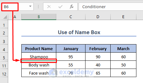
4. Unhide Specific Row Using Name Box in Excel
It’s quite easy to spot the hidden rows in a spreadsheet using the name box.
Name Box: In Excel, the Name Box alludes to an infobox on one side of the formula bar. The Name Box typically shows the location of the “dynamic/active cell” on the worksheet.
Steps:
➣In the Name Box next to the formula bar, type cell B6 which we want to unhide, and then press Enter. In the following picture, the green line means cell B6 is now selected.
➣Then, simply go to the Home tab > Format > Hide and Unhide > Unhide Rows.
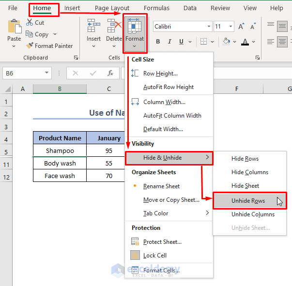
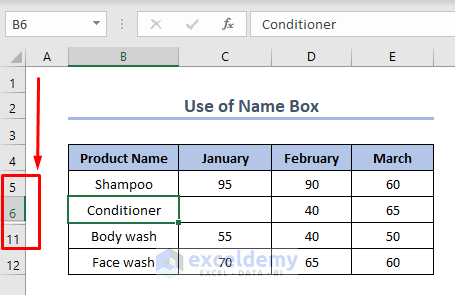
➣Now, we can see the whole row for cell B6 is visible.
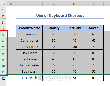
5. Disclose Rows with Keyboard Shortcut
We can show all the hidden rows with a keyboard shortcut.
Steps:
➣Firstly, select the rows including the row above and below we want to unhide. Then, press t Ctrl, Shift, 9 these three keys together from the keyboard.
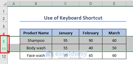
➣Pressing this key combination displays any hidden rows that intersect the selection.
Read More: Shortcut to Unhide Rows in Excel
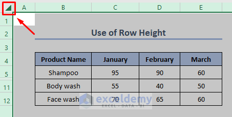
6. Make Rows Visible by Changing the Excel Row Height
We can easily unhide the rows by changing the Excel row height.
Steps:
➣Click the top left corner and select the whole spreadsheet.
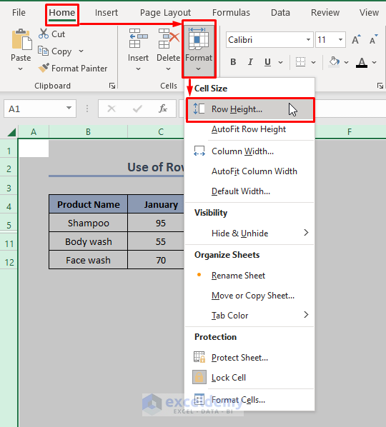
➣After that, go to the Home tab in the ribbon then the Format option. This option is found in the top-right of the Excel window in the “Cells” portion of the toolbar. There will be a drop-down menu. Select Row Height.
➣This will open a pop-up window with a blank text field in it. Enter a row height into the pop-up window text field. Here, I’m entering 18.
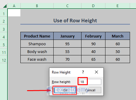
➣This will apply the changes to all the rows in the table and show all the rows that have been “hidden” by the height property.
7. Show All Hidden Rows in Whole Excel Spreadsheet
Assume we need to unhide all rows in the whole spreadsheet.
Steps:
➣Click here, in the top left corner, to unhide all rows in the whole spreadsheet. The entire sheet has been highlighted at this point.

➣Select the Unhide option from the right-click menu on the row headings section, and all rows in the spreadsheet will become visible.
Read More: Unhide All Rows Not Working in Excel
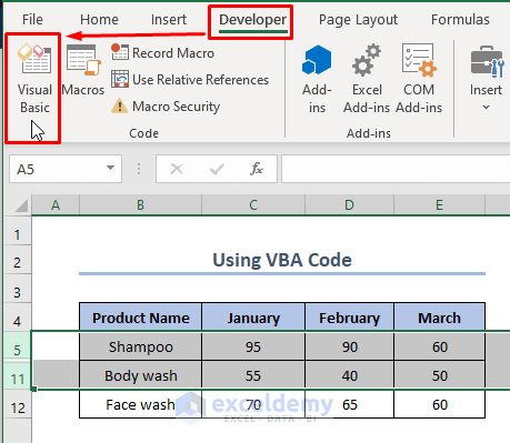
8. Unhide Rows Using VBA Code in Excel
Likewise the above dataset, we are going to use a VBA code to unhide all the rows in Excel.
Steps:
➣To start with, we must choose the rows we need to unhide. We can do it by choosing one row above and one beneath the row or rows we need to unhide. Go to the Visual Basic from Developer tab in the ribbon. This will open the visual basic editor.
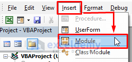
➣Click the Insert drop-down and select ‘Module’. This will insert a new module window.
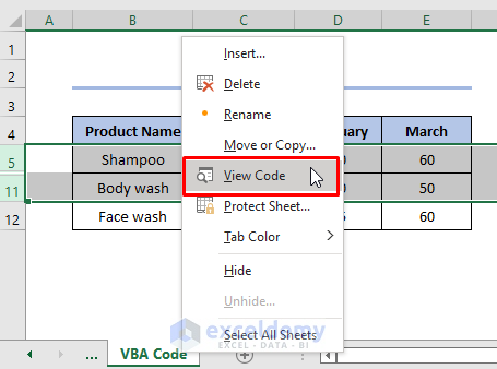
➣Or, just right-click on the spreadsheet bar. Go to View Code.
➣After that, write the VBA code.
VBA Code:
Sub UnhideAllRows()
Selection.EntireRow.Hidden = False
End Sub
➣Copy and paste the VBA code in the window. Then click on Run or use the keyboard shortcut (F5) to execute the macro code.
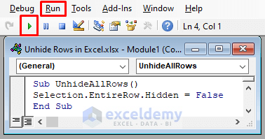
➣And finally, all the hidden rows will unhide in the worksheet.
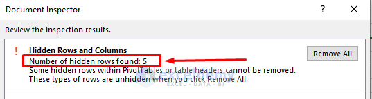
Check the Number of Hidden Rows
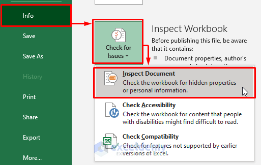
Excel has a feature called ‘Inspect Document‘ that allows you to quickly scan a workbook and get information about it. One of the things you can do using ‘Inspect Document‘ is to quickly see how many hidden columns or rows are in the worksheet. This could be beneficial if you receive a workbook from someone and want to inspect it fast. The steps to examine the total number of hidden columns or hidden rows are as follows.
Steps:
- Start by opening the workbook.
- Select the File tab.
- Go to the Info section.
- Click the ‘Check for Issues‘ drop-down (next to the Inspect Workbook text) in the Info choices.
- Click on Inspect Document.
- Make sure the Hidden Rows and Columns option is enabled in the Document Inspector. Then, click the Inspect button.
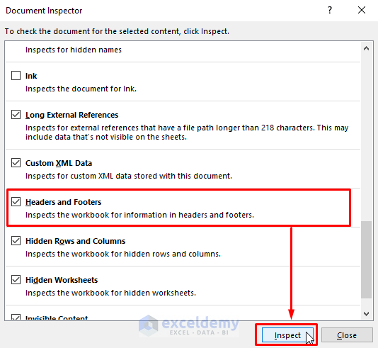
- This will show you the total number of hidden rows and columns.
Reasons Why Rows in Excel Cannot Be Unhidden
If you find difficulty in unhiding columns in your worksheets, it’s most probable in light of one of the accompanying reasons.
- Protected Worksheet
The first thing to check when the Hide and Unhide functions in Excel are disabled (grayed out) is worksheet protection.
Check the Review tab > Changes group to see if the Unprotect Sheet button is available (this button appears only in protected worksheets; in an unprotected worksheet, there will be the Protect Sheet button instead). So, if the Unprotect Sheet button appears, click it.
Click the Protect Sheet button on the Review tab, choose the Format rows box, then click OK to keep the worksheet protected but allow hiding and unhiding rows the selection.
- Small Row height, but Not Zero
Check the height of the rows. If the worksheet isn’t protected but specific rows can’t be unhidden.
- Filtered out Rows
When your worksheet’s row numbers become blue, it means that some rows have been filtered out. Simply remove all filters from a sheet to reveal such rows.
Tips:
We can unhide all cells in Excel. To unhide all rows and columns, select the entire spreadsheet as clarified above, and afterward press Ctrl + Shift + 9 to show stowed away rows and Ctrl + Shift + 0 to show stowed away columns.
Download Practice Workbook
You can download the workbook and practice with them.
Conclusion
By following these methods, you can easily unhide rows in your workbook. All these methods are simple, fast, and reliable. Hope this will help you! If you have any questions, suggestions, or feedback please let us know in the comment section.
Related Articles
<< Go Back to Hide Rows | Rows in Excel | Learn Excel
Get FREE Advanced Excel Exercises with Solutions!
