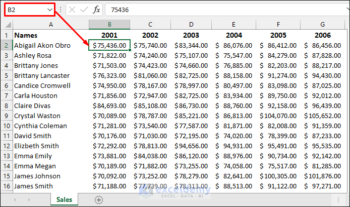
Imagine you have the following dataset containing sales made by employees in different years.
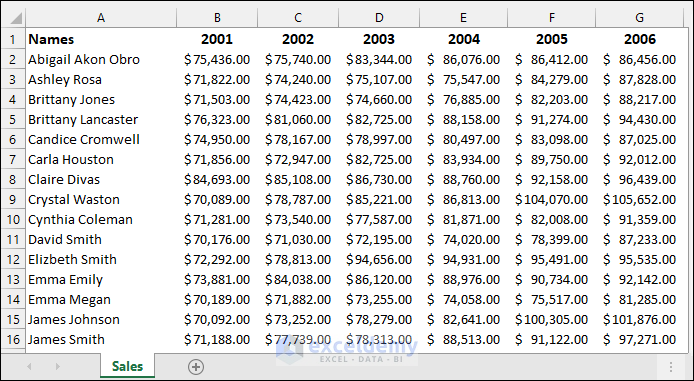
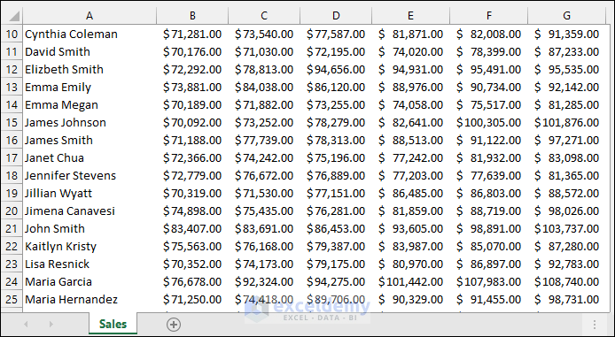
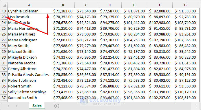
If you try to scroll down through the data, then you won’t see the years in the top row visible anymore. This makes it a bit difficult to understand the data.
Method 1 – Lock Top Row in Excel When Scrolling
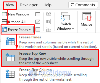
- Scroll up so the first row is visible.
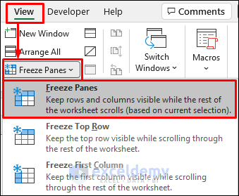
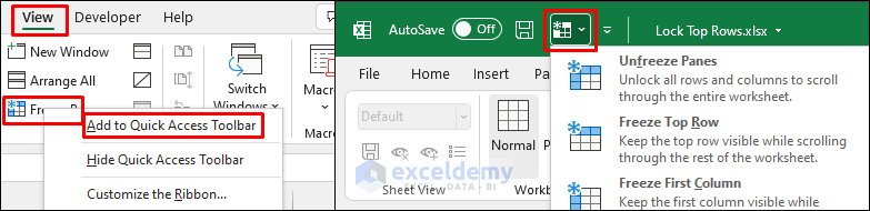
- Select the View tab.
- Go to Freeze Panes and choose Freeze Top Row from the drop-down list.
The top row will not move when you start scrolling down.
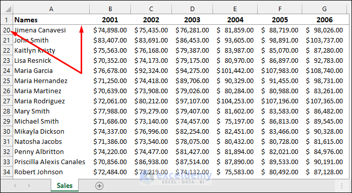
But if Row 10 was at the top, then it will be locked instead. Moreover, you won’t be able to see rows 1 to 9.
Read More: How to Lock Cells in Excel When Scrolling
Method 2 – Freeze Multiple Top Rows in Excel
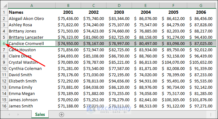
Let’s assume you want to lock the top five rows. Follow these steps:
- Select cell A6 or the row header for row 6.
- Select View, Freeze Panes, and then the Freeze Panes option in the drop-down.
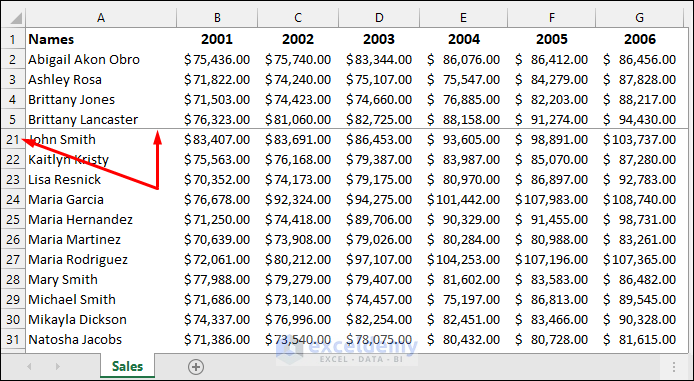
The top five rows won’t move when you scroll down.
Read More: How to Unlock Cells in Excel When Scrolling
Method 3 – Hide and Lock Top Rows in Excel
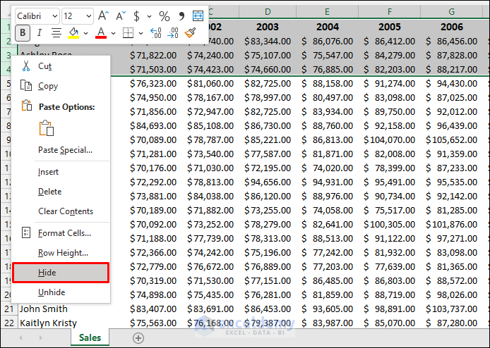
- Select the first few rows.
- Right-click.
- Select Hide.
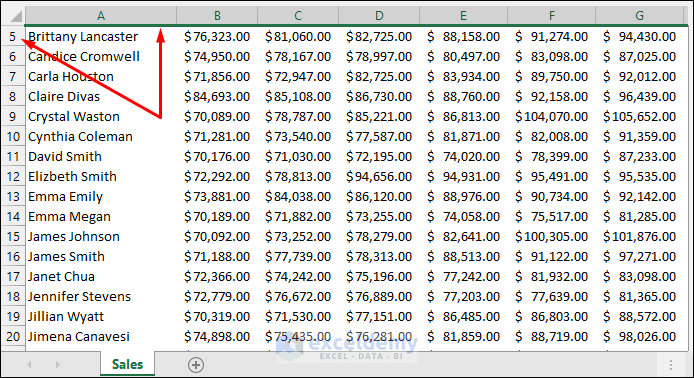
- You will see a solid green border at the top after hiding the rows. Now, row 5 is visible at the top instead of row 1.
- Select View >> Freeze Panes >> Freeze Top Row as in method 1.
- Unhide the hidden rows.

Do not select the Freeze Panes option if there are hidden rows. Otherwise, an arbitrary number of rows and columns will be locked.
Read More: Unfreeze Rows in Excel
Method 4 – Lock the Top Rows and Left Columns
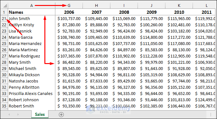
If you lock the top row, it won’t move when you scroll down. But, if you scroll horizontally, you won’t see the employee names visible.
Let’s fix this problem.
- Select cell B2, since it’s right below the top row and immediately right to the first column.
- Select View >> Freeze Panes >> Freeze Panes as earlier. The top row and the first column won’t move when you scroll horizontally or vertically.
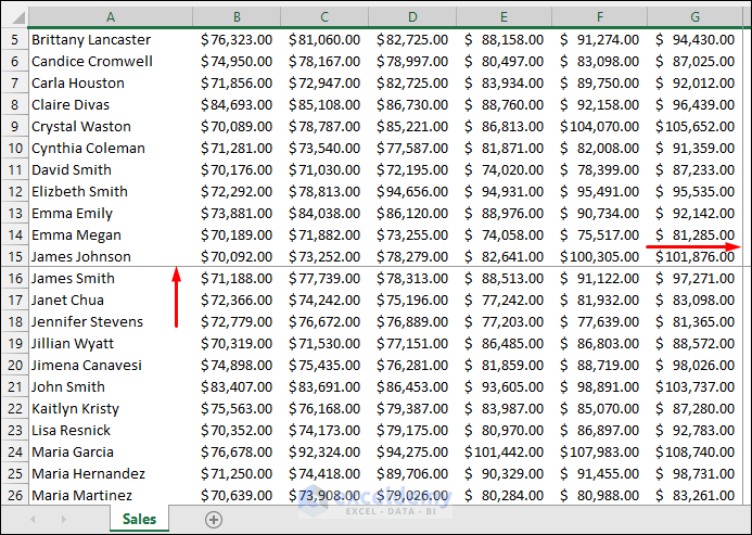
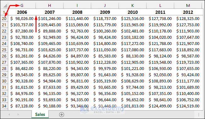
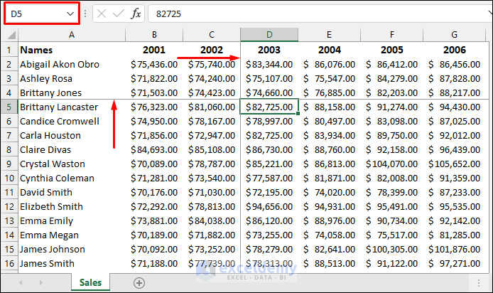
Now assume you want to lock the top four rows and the first three columns. You need to determine the cell right below row 4 and immediately right to the 3rd column. As cell D5 fulfills the criteria, select cell D5. Repeat the process as above.
Finally, you will get the desired result as shown in the picture below.
Read More: How to Unfreeze Columns in Excel
Unlock Top Rows in Excel
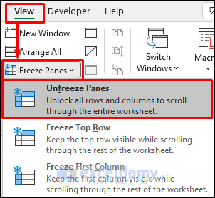
In the Freeze Panes drop-down, you will get an Unfreeze Panes to unlock the rows as shown below if you have any frozen rows or columns.
Read More: How to Freeze Top Row in Excel
Things to Remember
Before using the Freeze Panes command,
- Select the row just below the row that you want to lock.
- Select the column immediately right to the column that you want to lock.
- Select the cell just below the rows and immediately after the columns that you want to lock.
Download Practice Workbook
You can download the practice workbook from the download button below.
Related Article
- How to Freeze Top Two Rows in Excel
- How to Freeze Top 3 Rows in Excel
- How to Freeze Columns in Excel
- How to Freeze 2 Columns in Excel
- How to Freeze First 3 Columns in Excel
- How to Freeze Random Selection in Excel
<< Go Back to Freeze Panes | Learn Excel
Get FREE Advanced Excel Exercises with Solutions!
