Finding the max value and corresponding cell means looking for the maximum value(s) from a dataset and returning the cell location of the value.
In this tutorial, you will learn how to find the max value and corresponding cell in Excel.
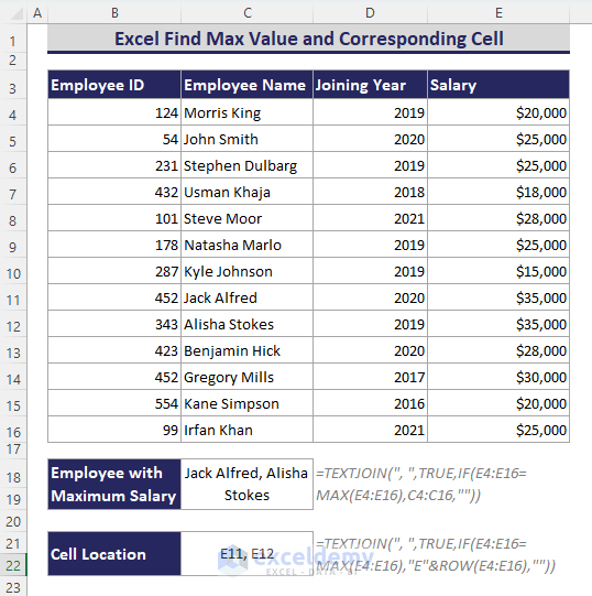
Look at the following image. Here we have an employee dataset with their ID, name, joining year, and salary. We figured out the employee name with the highest salary. And also we got the cell location of those values.
 Finding the max value and corresponding cells can be done by using Excel formulas and VBA code. Some Excel formulas will return the first max value with the corresponding cell from a dataset. Some other Excel formulas can return all the corresponding cells with the maximum value. We have also shown how to determine the max value and corresponding cell based on criteria.
1. Using Excel Formula to Find First Max Value and Corresponding Cell
By Combining Excel INDEX and MATCH Functions with other Excel Functions such as MAX, LARGE, AGGREGATE, and SUBTOTAL functions, we will find the first maximum value and corresponding cell in a single dataset.
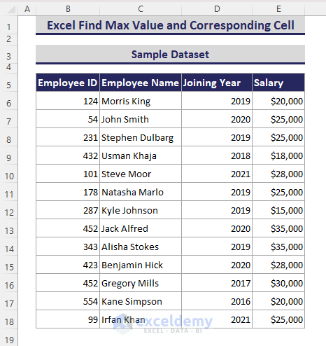
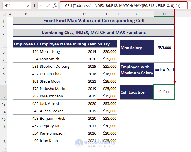
Here we are considering the below sample dataset containing Employee ID, Employee Name, Joining Year, and Salary. There are Jack Alfred and Alisha Stokes in the C13 and C14 cell who get the maximum salary of $35,000. However, the INDEX-MATCH formula returns only Jack Alfred since it is the first value in the dataset.
We can determine the maximum salary by applying the MAX function. We will use INDEX-MATCH formula along with the MAX function to extract the name of the employee who gets the maximum salary. Later, the CELL function can be applicable to achieve the cell reference of maximum salary.
Step 1: Finding Max Salary
The steps required steps are as follows:
- Initially, we obtain $35,000 in the H5 cell by inserting the formula below.
=MAX(E6:E18)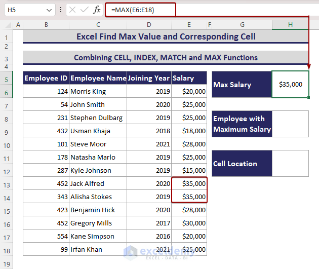
To get the Max value in the cell H5, you can also use any of the following formulas and these will give you the same output:
=LARGE(E6:E18,1)=AGGREGATE(4,6,E6:E18)=SUBTOTAL(4,E6:E18)Step 2: Finding Employee Name with Maximum Salary
Then, we get Jack Alfred in the H8 cell, the employee who gets the maximum salary with the formula as follows. But didn’t pick Alisha Stokes who also gets the max salary of $35000.
=INDEX(B6:E18,MATCH(MAX(E6:E18),E6:E18,0),2)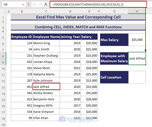
The alternative formulas to find the employee name (in cell H8) with maximum salary are:
=INDEX(B6:E18,MATCH(LARGE(E6:E18,1),E6:E18,0),2)=INDEX(B6:E18,MATCH(AGGREGATE(4,6,E6:E18),E6:E18,0),2)=INDEX(B6:E18,MATCH(SUBTOTAL(4,E6:E18),E6:E18,0),2)Step 3: Finding the Corresponding Cell Location with the Maximum Value
In the cell H11, we input this formula:
=CELL("address", INDEX(B6:E18, MATCH(MAX(E6:E18), E6:E18, 0),4))
This formula shows the cell reference $E$13. Because the E13 cell stores the first maximum value of $35000 in the Salary column.
=CELL("address",INDEX(B6:E18,MATCH(LARGE(E6:E18,1),E6:E18,0),4))=CELL("address",INDEX(B6:E18,MATCH(AGGREGATE(4,6,E6:E18),E6:E18,0),4))=CELL("address",INDEX(B6:E18,MATCH(SUBTOTAL(4,E6:E18),E6:E18,0),4))=ADDRESS(MATCH(MAX(E6:E18), E6:E18, 0) + ROW(E5), 5)="$E$"&MATCH(MAX(E6:E18),E6:E18,0)+ROW(E5)Formula Breakdown
- INDEX(B6:E18,MATCH(MAX(E6:E18),E6:E18,0),2) => The MAX(E6:E18) returns 35000, the maximum value in the E6:E18 range.
- INDEX(B6:E18,MATCH(35000,E6:E18,0),2) => The MATCH(35000,E6:E18,0) returns 8 which is the row number of the selected range.
- INDEX((B6:E18,8,2) => The INDEX function returns the $E$13 cell which is the 8th row and 2nd column of the B6:E18 range.
2. Finding Max Value and Corresponding Cell from Multiple Excel Ranges
The MAX function not only considers adjacent cells but also non-adjacent cells. The function also finds the maximum value and corresponding cell location in Excel.
- Inserting the formula with non-adjacent cells, we achieve $35,000 in the H5 cell.
=MAX(E6:E12,E15:E20)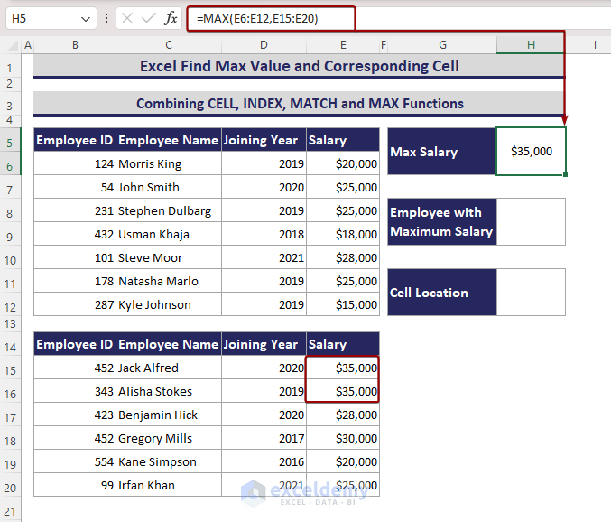
- Next, we get the Jack Alfred in the H8 cell by applying the formula as follows.
=INDEX(B6:E20,MATCH(MAX(E6:E12,E15:E20),E6:E20,0),2)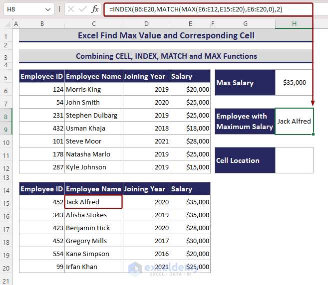
- Further, we get $E$15 cell reference of the highest value by applying the following formula.
=CELL("address",INDEX(B6:E20,MATCH(MAX(E6:E12,E15:E20),E6:E20,0),4))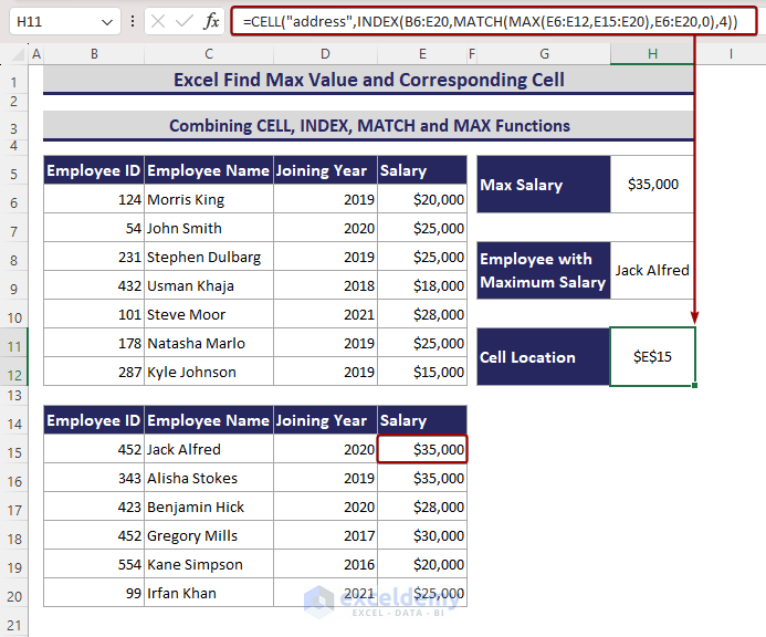
Read More: How to Find Max Value in Range with Excel Formula
3. Using Excel Formulas to Find Corresponding Multiple Cells with Max Value
Unlike the previous method, in this section, we will find out multiple maximum values and their corresponding cell location by applying combinations of the TEXTJOIN-IF-MAX formula and the FILTER-MAX formula in Excel.
3.1 Combining TEXTJOIN and IF Functions
Here, we will combine TEXTJOIN and IF Functions to find corresponding multiple cells with Max Value.
By applying the MAX function we get the maximum value from the Salary range. Then IF function picks up the employee names who get the maximum salary. After that, the TEXTJOIN function adds all the names with a delimiter.
Please follow the necessary steps:
- By applying the following formula, we get Jack Alfred, Alisha Stokes in the H5 cell.
=TEXTJOIN(", ", TRUE, IF(E6:E18=MAX(E6:E18), C6:C18, ""))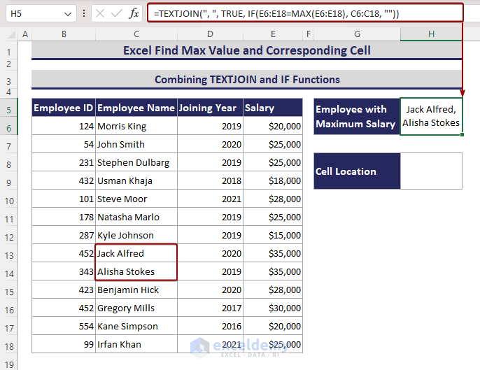
- Lastly, we obtain the E13, E14 cell references by inserting the formula as follows.
=TEXTJOIN(", ", TRUE, IF(E6:E18=MAX(E6:E18), "E" & ROW(E6:E18), ""))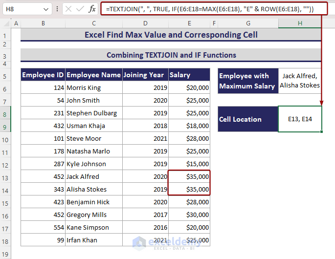
3.2 Merging FILTER, MAX and TEXTJOIN Functions
The MAX function determines the maximum value. Then, the FILTER function filters those maximum values and shows them.
Please check out the required steps:
- Enter the following formula in Cell G7 and you will see the employee name with maximum salary.
=FILTER(C6:C18,E6:E18=MAX(E6:E18))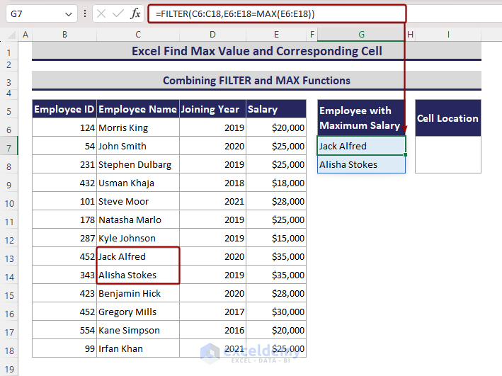
- Now enter the following formula in cell I7 and you will get the corresponding cell location of max values.
=TEXTJOIN(", ", TRUE, IF(E6:E18=MAX(E6:E18), "E" & ROW(C6:C18), ""))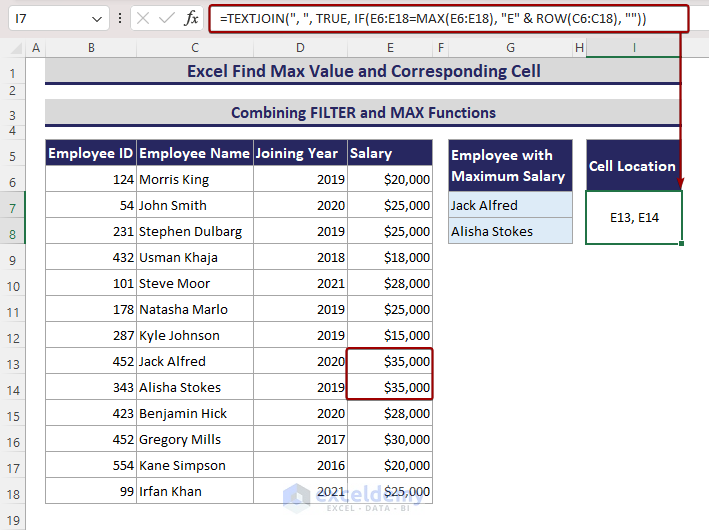
4. Finding Corresponding Multiple Cells with Max Value Based on Criteria
In this section, we will discuss how to find multiple maximum values and their corresponding cell references based on criteria. The combination of the MAX, IF, TEXTJOIN and TEXTSPLIT functions is applicable for single and multiple criteria; Besides, the combination of IF, MAXIFS, TEXTJOIN, and TEXTSPLIT functions is also useful for multiple criteria.
4.1 Combining MAX, IF, TEXTJOIN and TEXTSPLIT Functions for Single Criterion
Suppose we are likely to find the maximum salary of employees who joined after 2018. Using the MAX, IF, TEXTJOIN, and TEXTSPLIT functions we can find the multiple employees with max salary and their corresponding cell references based on a single criterion.
Please follow the necessary steps below:
- Enter the following formula in cell G9 and press Enter. You will get the employee names in an array format.
=IFERROR(TEXTSPLIT(TEXTJOIN(",", TRUE,IF((D6:D18 > H5)*(E6:E18 = MAX(IF(D6:D18 > H5, E6:E18))), C6:C18, ""),),,","),"")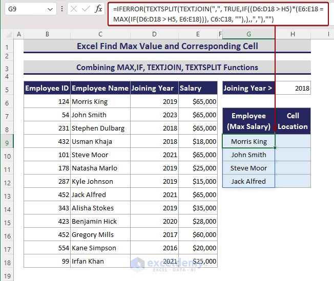
- Now enter the following formula in cell H9 and you will get the corresponding cell location of max values.
=IFERROR(CELL("address",INDEX($E$6:$E$18, MATCH(G9, $C$6:$C$18, 0),1)),"")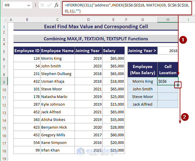
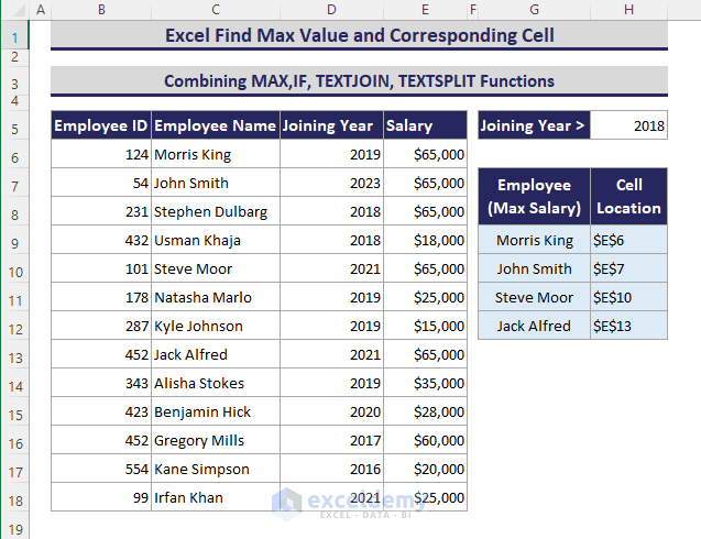
- Further, we get the cell locations of maximum salary by dragging the Fill Handle tool.
4.2 Joining MAX, IF, TEXTJOIN and TEXTSPLIT Functions for Multiple Criteria
Assume, we want to find the employees with the maximum salary who joined between 2020 to 2023. Using Excel MAX, IF, TEXTJOIN, and TEXTSPLIT functions we can find multiple employees with max salary and their corresponding cell references based on multiple criteria.
Please follow the necessary steps below:
- Write the following formula in cell G10 and press Enter. You will get the employee names in an array format.
=IFERROR(TEXTSPLIT(TEXTJOIN(",", TRUE, IF((D6:D18 >=H5)*(D6:D18 <=H6), IF(E6:E18 = MAX(IF((D6:D18 >=H5)*(D6:D18 <=H6), E6:E18)), C6:C18, ""), ""),),,","),"")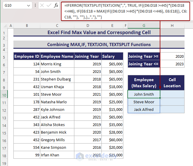
- Now input the following formula in the H10 cell and you will get the corresponding cell reference of max values.
=IFERROR(CELL("address",INDEX($E$6:$E$18, MATCH(G10, $C$6:$C$18, 0),1)),"")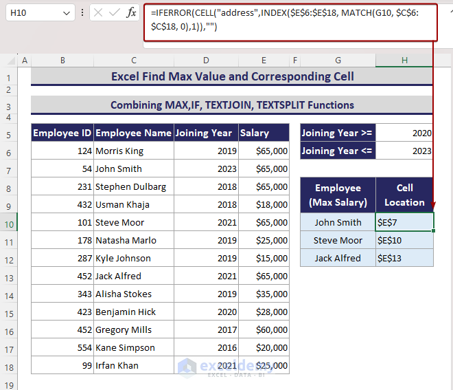
4.3 Merging IF, MAXIFS, TEXTJOIN and TEXTSPLIT Functions for Multiple Criteria
Like the previous method, we can also find multiple employees with max salary and their corresponding cell references based on multiple criteria. Here, we will use Excel MAXIFS, IF, TEXTJOIN, and TEXTSPLIT functions.
Please follow the necessary steps below:
- Insert the following formula in cell G10 and press Enter. You will get the employee names in an array format.
=IFERROR(TEXTSPLIT(TEXTJOIN(",", TRUE, IF((D6:D18 >=H5)*(D6:D18 <=H6), IF(E6:E18 =MAXIFS(E6:E18, D6:D18, ">="&H5, D6:D18, "<="&H6), C6:C18, ""), "")),,","),"")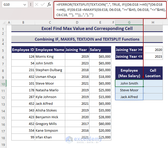
- Now write the following formula in the H10 cell and you will get the corresponding location that contains max values.
=IFERROR(CELL("address",INDEX($E$6:$E$18, MATCH(G10, $C$6:$C$18, 0),1)),"")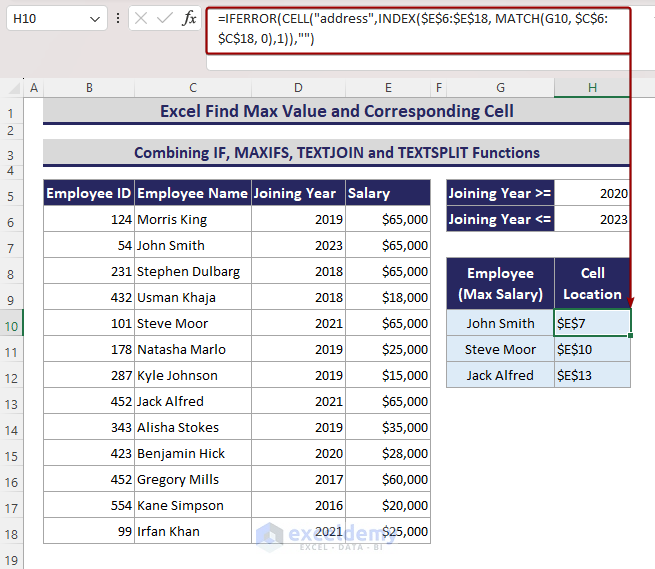
Read More: How to Find Maximum Value in Excel with Condition
5. Using VBA Macro to Find Multiple Max Values and Corresponding Cell Locations
In this section, you will learn to use the VBA Macro to find the max value and corresponding cell in Excel. As you know, Excel functions and formulas find max values but fail to determine corresponding cell locations from multiple ranges.
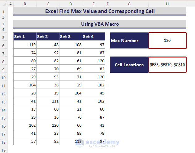
We are considering the dataset as follows which contains some random numbers and 120 is the highest number that is located in E8, E10, and C16 cells.
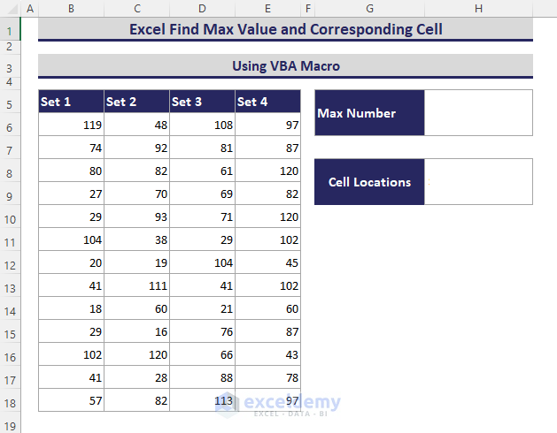
- Now, write the following VBA code in the Module and click on the Run command.
Sub Find_Multiple_Max_Values_And_Addresses_from_Range()
Dim rng As Range
Dim maxVal As Double
Dim results() As String
Dim i As Long
Dim CellAddress As String
Dim outputRange As Range
Set rng = Application.InputBox("Select a range:", Type:=8)
ReDim results(1 To rng.Cells.Count)
i = 1
maxVal = Application.WorksheetFunction.Max(rng)
For Each cell In rng
If cell.Value = maxVal Then
results(i) = cell.Address
i = i + 1
End If
Next cell
If i > 1 Then
ReDim Preserve results(1 To i - 1)
CellAddress = Join(results, ", ")
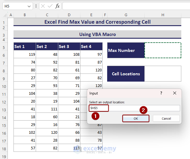
Set outputRange = Application.InputBox("Select an output location:", Type:=8)
outputRange.Value = maxVal
outputRange.Offset(2, 0).Value = CellAddress
End If
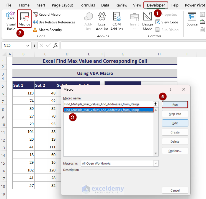
End Sub- Then Click as follows: Developer => Macro.
- Next, you will get a Macro dialog box and click Find_Multiple_Max_Values_and_Addresses_from_Range => Run.
Code Breakdown
- Initially, we created a sub-procedure named Find_Multiple_Max_Values_And_Addresses_from_Range.
Sub Find_Multiple_Max_Values_And_Addresses_from_Range()
[Code]
End Sub- Then, we insert the input range using the Application.InputBox property with the rng variable. Also, declaring rng as the Range variable.
Dim rng As Range
Set rng = Application.InputBox("Select a range:", Type:=8)- Next, we count the cells of the rng range using Cells.Count property and take the input range in an array. So, we declare results() As String variable.
Dim results() As String
ReDim results(1 To rng.Cells.Count)- After that, by inserting the Application.WorksheetFunction.Max(rng) statement, we apply Excel MAX function to figure out the maximum value.
Dim maxVal As Double
maxVal = Application.WorksheetFunction.Max(rng)- Now, we must run a For loop to consider all the cell values from the rng range from where cell locations will be extracted based on a logical statement.
For Each cell In rng
[Logical Statement]
Next cell- Further, picking up the value of cell using cell.Value property and compare it with the maximum value. So, initialization with the 1st value with statement i = 1 and increment takes place gradually with i = i+1 statement. If it is maximum then get the cell reference using cell.Address property. In the meantime, all the cell locations containing maximum values are restored in the results(i) array.
Dim i As Long
i = 1
If cell.Value = maxVal Then
        results(i) = cell.Address
        i = i + 1
End If- If the value of results(i) is more than 1 then combine the cell references with the Excel Join property. The CellAddress is the assigned variable which is String type.
Dim CellAddress As String
If i > 1 Then
    ReDim Preserve results(1 To i - 1)
    CellAddress = Join(results, ", ")
End If- Finally, we select the output locations by writing outputRange variable with Application.InputBox property. So, we declare outputRange variable as Range. outputRange.Value and outputRange.Offset(2, 0).Value properties result in maximum value and corresponding cell references in Excel.
Dim outputRange As Range
Set outputRange = Application.InputBox("Select an output location:", Type:=8)
outputRange.Value = maxVal
outputRange.Offset(2, 0).Value = CellAddress- Thus, an Input dialog box appears and selects $B$6:$E$18 range => OK.

- Next, another Input dialog box appears and selects the $H$5 range => OK.
- Therefore, we obtain the max value of 120 in the H6 cell and their cell locations $E$8, $E$10, $C$16 in the worksheet.
Download Practice Workbook
Conclusion
In short, the INDEX-MATCH formula with MAX, LARGE, AGGREGATE, or SUBTOTAL functions returns the first max value and the corresponding cell only. On the contrary, a combination of the TEXTJOIN-IF and FILTER-MAX-TEXTJOIN formulas returns two or multiple data for max values and corresponding cells. Besides, the combination of the MAX, IF, TEXTJOIN, and TEXTSPLIT Functions is useful when single and multiple criteria are applied. Further, the combination of IF, MAXIFS, TEXTJOIN, and TEXTSPLIT functions is also applicable to multiple criteria. Further, VBA Macro is essential to find out the maximum values and their cell locations from two or multiple ranges. Hope this article makes your learning easier. Please leave your thoughts, suggestions, and any queries in the comment section.
Related Articles
- Set a Minimum and Maximum Value in Excel
- Excel MIN and MAX in Same Formula
- How to Cap Percentage Values Between 0 and 100 in Excel
<< Go Back to Excel MAX Function | Excel Functions | Learn Excel
Get FREE Advanced Excel Exercises with Solutions!
