Here is a data set with the Names of some students, and their Marks in Physics and Chemistry.
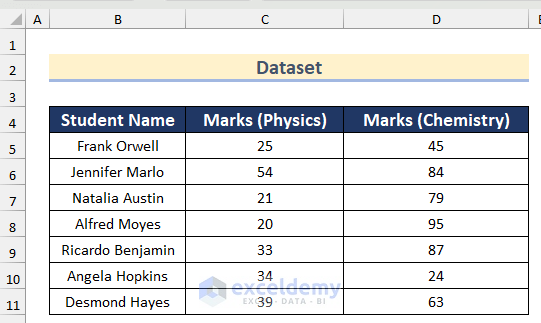
Let’s try to combine the IF, INDEX, and MATCH functions in all possible ways from this data set.
Method 1 – Wrap INDEX-MATCH Within IF Function in Excel
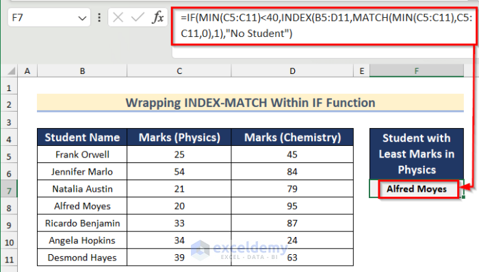
Let’s say we need to find the student with the lowest score in Physics, but only if that score is lower than 40. However, if it is not, then there is no need to find out the student and it will show “No Student”.
Steps:
- Select an empty cell, such as F7.
- Insert the following formula and press Enter:
=IF(MIN(C5:C11)<40,INDEX(B5:D11,MATCH(MIN(C5:C11),C5:C11,0),1),"No Student")- Since the lowest number in Physics is less than 40 (20 in this case), we have found the student with the least number. That is Alfred Moyes.
How Does the Formula Work?
- MIN(C5:C11) returns the smallest value in column C5:C11 (Marks in Physics). In this example, it is 20. See the MIN function for details.
- The formula becomes IF(20<40,INDEX(B5:D11,MATCH(20,C5:C11,0),1),”No Student”).
- As the condition within the IF function (20<40) is TRUE, it returns the first argument: INDEX(B5:D11,MATCH(20,C5:C11,0),1).
- MATCH(20,C5:C11,0) searches for an exact match of 20 in column C5:C11 (Marks in Physics) and finds one in the fourth row (In cell C8). So, it returns 4.
- The formula becomes INDEX(B5:D11,4,1). It returns the value from the 4th row and 1st column of the range B5:D11 (Data set excluding the Column Headers).
- That is the name of the student with the least number in Physics: Alfred Moyes.
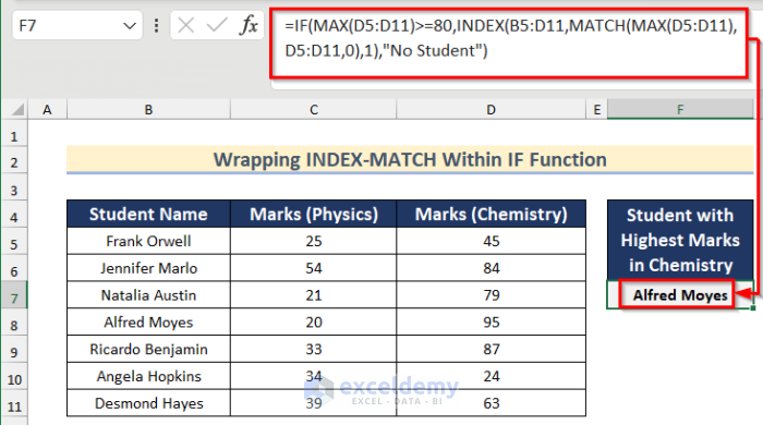
Take a moment to determine the formula to find out the student with the highest number in Chemistry, if the highest number is greater than or equal to 80. Otherwise, return “No student”.
Here’s the solution:
- Insert the following formula in Cell F7:
=IF(MAX(D5:D11)>=80,INDEX(B5:D11,MATCH(MAX(D5:D11),D5:D11,0),1),"No Student")- Press Enter.
Method 2 – Use IF Function within INDEX Function in Excel
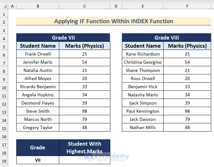
Consider the following dataset. It contains Physics results for students in two different grades.
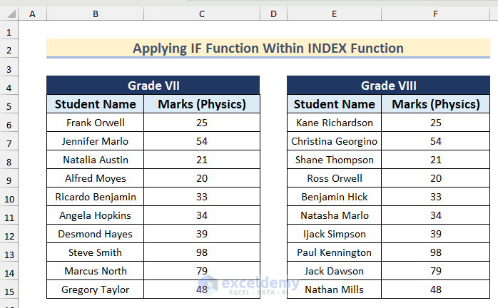
Now, we have Cell B19 in the worksheet that contains VII. We want to derive a formula that will show the student with the highest marks of Grade VII in the adjacent cell if B19 contains VII. However, if it contains VIII, the formula will show the student with the highest marks from Grade VIII.
Steps:
- Select Cell C19.
- Insert the following formula and press Enter:
=INDEX(IF(B19="VII",B6:C15,E6:F15),IF(B19="VII",MATCH(MAX(C6:C15),C6:C15,1),MATCH(MAX(F6:F15),F6:F15,1)),1)- Since there is VII in Cell B19, we are getting the student with the highest marks from Grade VII. That is Steve Smith, with 98 marks.
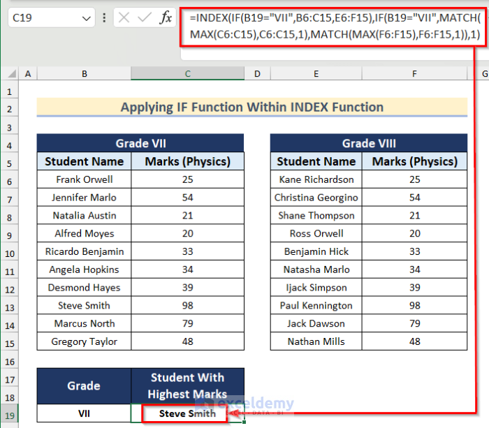
- However, if we enter VIII in B19, we will get the student with the highest marks from Grade VIII. That will be Paul Kennington.

How Does the Formula Work?
- IF(B19=”VII”,B6:C15,E6:F15) returns the range B6:C15 if cell B19 contains “VII”. Otherwise, it returns E6:F15.
- IF(B19=”VII”,MATCH(MAX(C6:C15),C6:C15,1),MATCH(MAX(F6:F15),F6:F15,1)) returns MATCH(MAX(C6:C15),C6:C15,1) if B19 contains “VII”. Otherwise, it returns MATCH(MAX(F6:F15),F6:F15,1).
- Therefore, when B19 contains “VII”, the formula becomes INDEX(B6:C15,MATCH(MAX(C6:C15),C6:C15,1),1).
- MAX(C6:C15) returns the highest marks from the range C6:C15 (Marks of Grade VII). It is 98 here.
- The formula becomes INDEX(B6:C15,MATCH(98,C6:C15,1),1).
- MATCH(98,C6:C15,1) searches for an exact match of 98 in column C6:C15. It finds one in the 8th row, in cell C13. It then returns 8.
- Finally, the formula now becomes INDEX(B6:C15,8,1). It returns the value from the 8th row and 1st column of the data set B6:C15: Steve Smith.
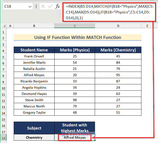
Method 3 – Apply IF Function within MATCH Function in Excel
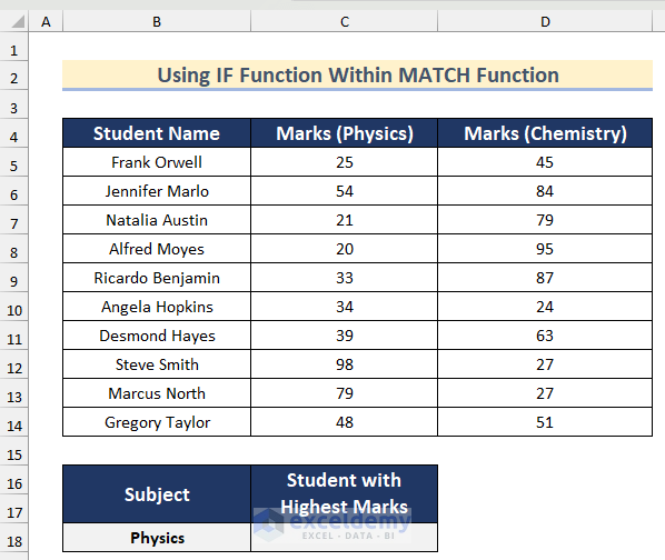
Let’s go back to our original data set, with the Marks of Physics and Chemistry.
Cell B18 of the worksheet contains the name of the subject: “Physics”. We will derive a formula that will show the student with the highest marks in Physics in the adjacent Cell if B18 has “Physics” in it. On the other hand, if it has “Chemistry”, it will show the student with the highest marks in Chemistry.
Steps:
- Select Cell C18.
- Insert the following formula and press Enter:
=INDEX(B5:D14,MATCH(IF(B18="Physics",MAX(C5:C14),MAX(D5:D14)),IF(B18="Physics",C5:C14,D5:D14),0),1)- The results show Steve Smith, because Cell B18 contains “Physics” and he has the highest marks in Physics.
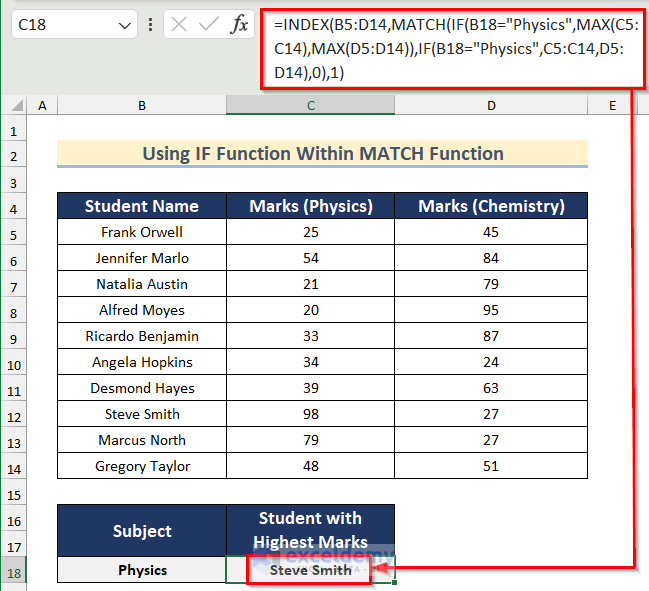
- If we change cell F7 to “Chemistry”, it will show Alfred Moyes, the highest marks getter in Chemistry.
How Does the Formula Work?
- IF(B18=”Physics”,MAX(C5:C14),MAX(D5:D14)) returns MAX(C5:C14) if F7 contains “Physics”. Otherwise, it returns MAX(D5:D14).
- IF(B18=”Physics”,C5:C14,D5:D14) returns C5:C14 if B18 contains “Physics”. Otherwise, it returns D5:D14.
- So, if B18 contains “Physics”, the formula becomes INDEX(B5:D14,MATCH(MAX(C5:C14),C5:C14,0),1).
- MAX(C5:C14) returns the highest marks from the range C5:C14 (Marks of Physics). It is 98 here.
- The formula becomes INDEX(B5:D14,MATCH(98,C5:C14,1),1).
- MATCH(98,C5:C14,1) searches for an exact match of 98 in column C5:C14. It finds one in the 8th row, in cell C12. So, it returns 8.
- The formula now becomes INDEX(B5:D14,8,1). It returns the value from the 8th row and 1st column of the data set B5:D14: Steve Smith.
Things to Remember
- Always set the 3rd argument of the MATCH function to 0 if you want an exact match.
- There are a few alternatives to the INDEX-MATCH formula, like the FILTER, VLOOKUP, and XLOOKUP functions.
- Among the alternatives, the FILTER function returns all the values that match the criteria, but it’s available in Microsoft 365 only.
Download Practice Workbook
You can download the workbook to practice yourself.
<< Go Back to INDEX MATCH | Formula List | Learn Excel
Get FREE Advanced Excel Exercises with Solutions!
