How to Move Data from One Cell to Another in Excel (5 Ways)

When working with Excel, it is a common scenario that we need data in a specific row or column, but we have inserted the data in other rows or columns. In this case, it is tiring to put the data again on the required rows or columns. Instead, we can simply move the inserted data to the required rows or columns. In this article, I will show you 5 suitable ways to move data from one cell to another.

Download Practice Workbook

You can download our practice workbook from here for free!

5 Suitable Ways to Move Data from One Cell to Another in Excel

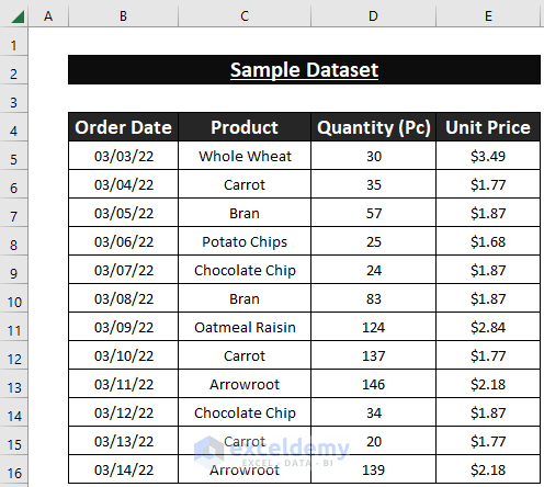
Say, we have a dataset of Product Sales containing Order Date, Product, Quantity (Pc), and Unit Price columns. Now, we want to move the Unit Price column (cells E4:E16) rightward (cells F4:F16). You can follow any of the ways given below to do this.

1. Dragging and Dropping with Mouse

The quickest way to move data from one cell to another is to use the drag and drop your left mouse button. Follow the steps below to do this.

📌 Steps:

• First and foremost, select cells E4:E16.
• Afterward, place your cursor on the right corner of your selection.
• As a result, a move cursor will appear.
• Now, left-click on your mouse and drag the selection to column F.

Thus, the entire selection will be moved to cells F4:F16. And, the outcome should look like this.

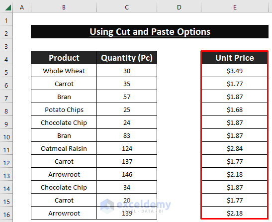
2. Using Cut and Paste Options

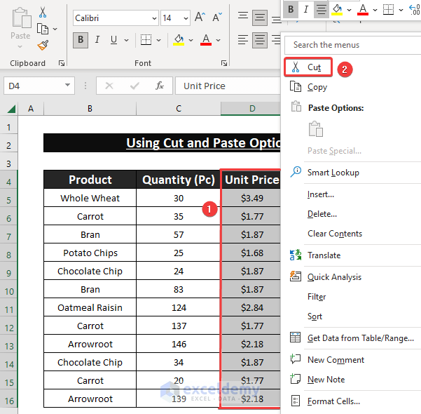
You can also use the cut-and-paste options to move data from one cell to another in Excel. Say, you have Unit Price data in D4:D16 cells which you want to move to E4:E16 cells. Go through the steps below to do this.

📌 Steps:

• First, select cells D4:D16.
• Following, click on your right mouse and choose the Cut option from the context menu.

• Afterward, click on cell F4 and right-click on your mouse button.
• Subsequently, choose the Paste option from the context menu.

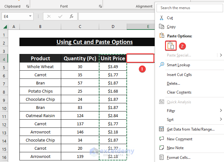
Thus, you will be able to move all your desired data from one cell to another. And, the final result should look like this.

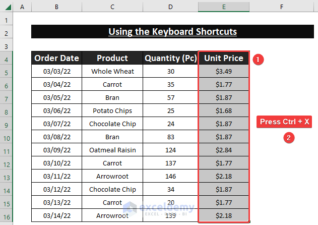
3. Using Keyboard Shortcuts to Move Data from One Cell to Another

Another quick way to move data from one cell to another is to use keyboard shortcuts. Follow the steps below to accomplish this.

📌 Steps:

• At the very beginning, select cells which you want to move (cells E4:E16 here).
• Following, press Ctrl + X.

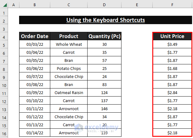
• Afterward, click on cell F4 and press Ctrl + V.

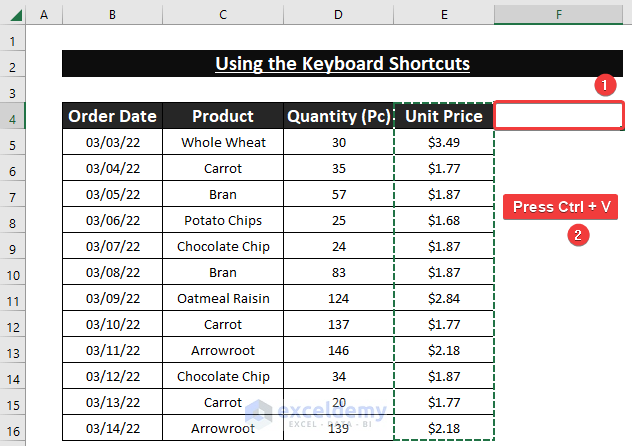
As a result, your task will be accomplished. And, for example, the outcome should look like this.

4. Using the Insert Cells Command

Besides, you can move data from one cell to another by using the Insert tool. Go through the steps below to accomplish this.

📌 Steps:

• First, select cells E4:E16.
• Following, go to the Home tab >> Cells group >> Insert tool >> Insert Cells… option.

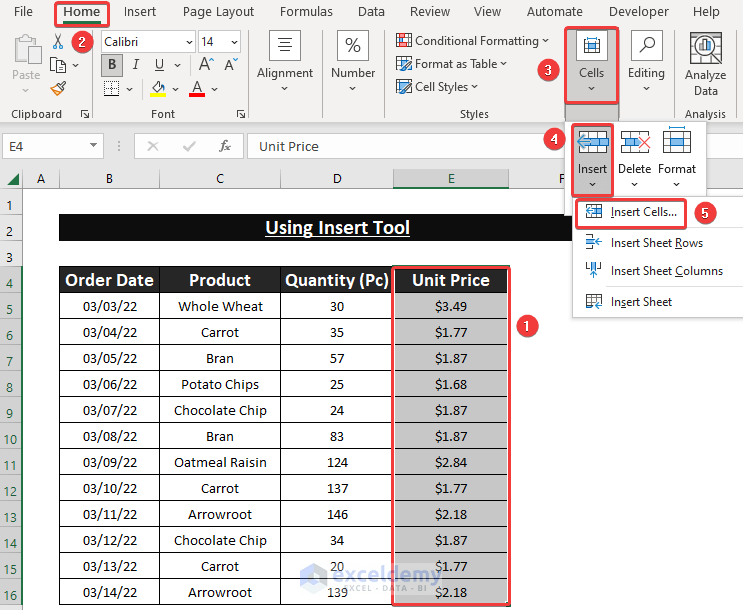
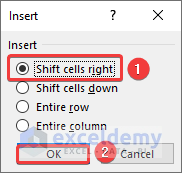
• As a result, the Insert window will appear.
• Subsequently, choose the option Shift cells right option and click on the OK button.

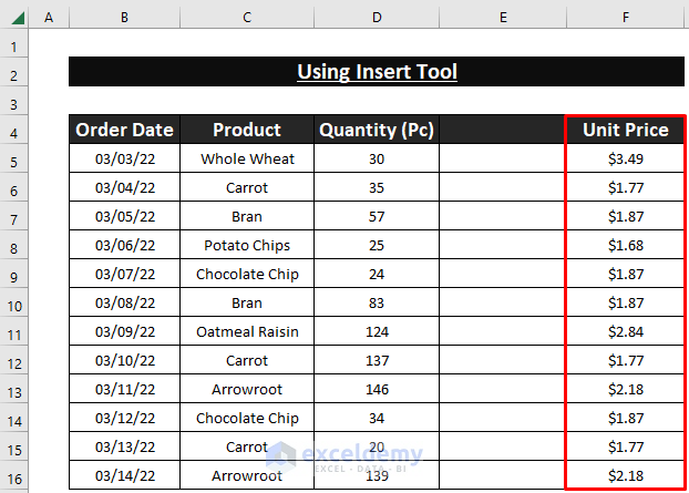
As a result, you will be able to move the selected data to your desired locations. And, the outcome should look like this.

5. Using a VBA Code to Move Data from One Cell to Another

Moreover, you can use a VBA code to move data from one cell to another. Follow the steps below to do this.

📌 Steps:

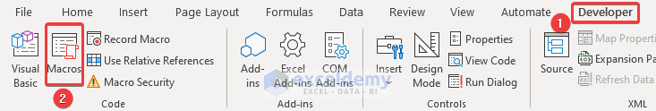
• First, go to the Developer tab >> Visual Basic tool.

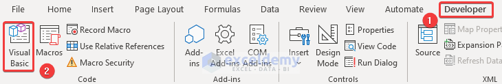
• As a result, the VB Editor window will appear.
• Following, go to the Insert tab >> Module option.

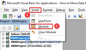
• As a result, a new module named Module1 will be created.
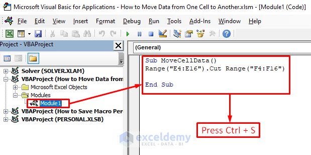
• Following, click on Module1 and write the following code in the code window.

Sub MoveCellData()
Range("E4:E16").Cut Range("F4:F16")
End Sub

• Subsequently, press Ctrl + S on your keyboard.

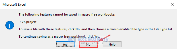
• As a result, a Microsoft Excel window will appear.
• Following, click on the No button.

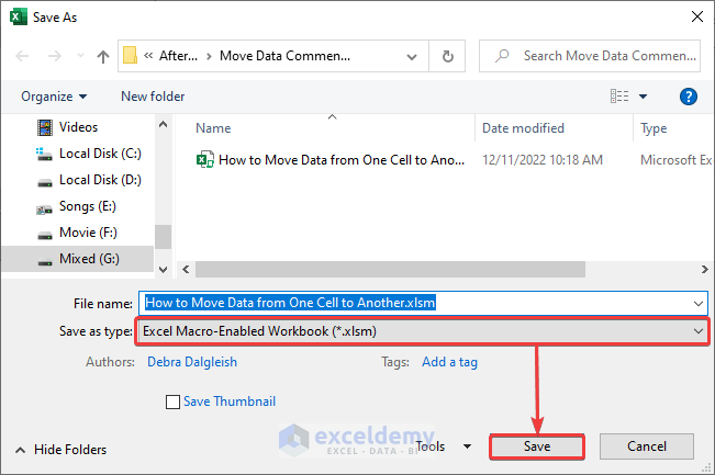
• As a result, the Save As dialogue box will appear.
• Following, choose the Save as type: as .xlsm file and click on the Save button.

• Afterward, go to the Developer tab again and click on the Macros tool.
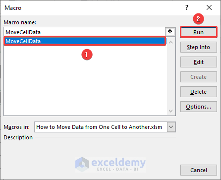
• As a result, the Macro window will appear.

• Following, choose the MoveCellData macro and click on the Run button.

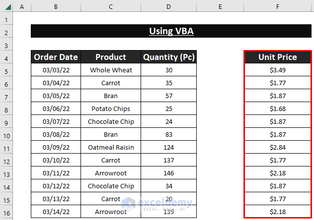
Thus, you will see cells E4:E16 shifted to F4:F16.

How to Copy Data from One Sheet to Another in Excel

Now, you might need to copy data from one sheet to another sheet in Excel sometimes. Follow the steps below to accomplish this.

📌 Steps:

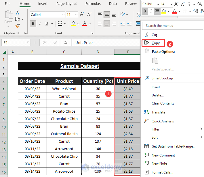
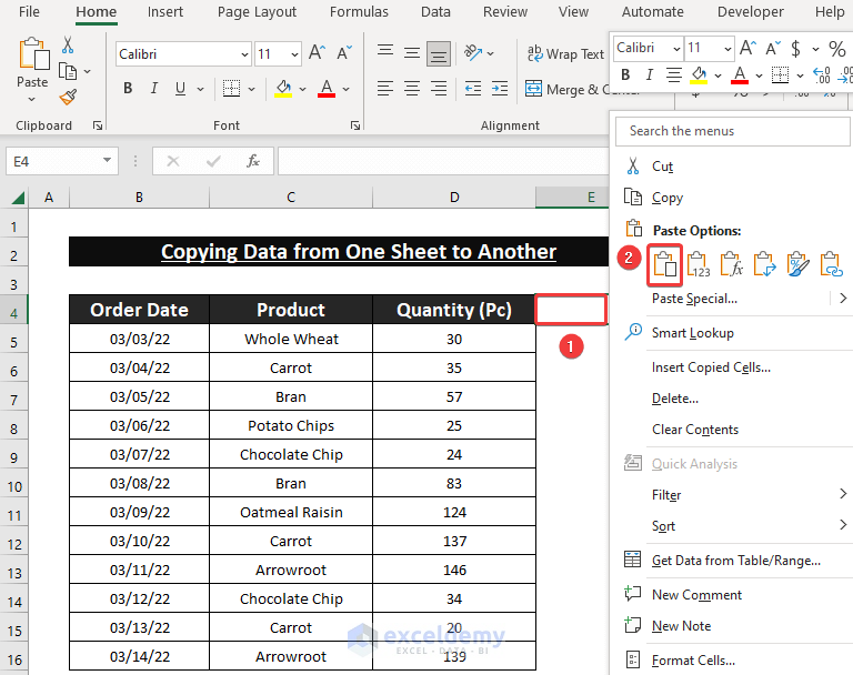
• First, select the cells you want to copy (cells E4:E16 here) from the sheet (Sample Dataset) from which you want to copy data.
• Subsequently, right-click on your mouse and choose the Copy option from the context menu.

• Afterward, click on the cell (cell E4 here) of the desired sheet where you want to paste the values.
• Following, right-click on your mouse and choose the Paste option from the context menu.

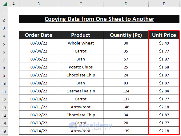
As a result, you will be able to acquire your desired result. And, the outcome would look like this.

Conclusion

So, in this article, I have shown you 5 suitable ways to move data from one cell to another in Excel. Read the full article carefully and practice accordingly. I hope you find this article helpful and informative. You are very welcome to comment here if you have any further questions or recommendations.

And, visit ExcelDemy to learn about many more Excel problem solutions, tips, and tricks. Thank you!