Excel Formula to Compare and Return Value from Two Columns

Excel is one of the significant applications used in both computers and mobile. We cannot think of a modern corporate house that does not use Excel. Working with Excel means lots of data, columns, and rows. In this article, we discuss the 4 Examples formula to compare two columns and return a value in Excel with proper illustrations.

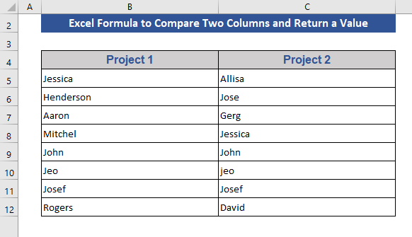
We will apply 4 different methods to compare two columns and return a value. We may need to use different data sets for different methods. Initially, we are taking data of some project managers’ names working on two projects.

1. Combining Formula with Excel IF and EXACT Functions to Compare Two Columns and Return Value

The IF function allows us to make logical comparisons between a value and our desire. This IF statement can have two results. The first result is if our comparison is True, and the second is if our comparison is False.

Syntax:

IF(logical_test, value_if_true, [value_if_false])

Argument:

logical_test – The desired condition we want to test.

value_if_true – The value we want to return if the result of logical_test is TRUE.

value_if_false – The value will return if the result of logical_test is FALSE.

1.1 Case-insensitive Approach

This approach is not case-sensitive. That means Jeo and jeo are considered the same.

Step 1:

• Go to Cell D5.
• Write the following formula:

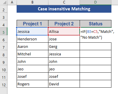
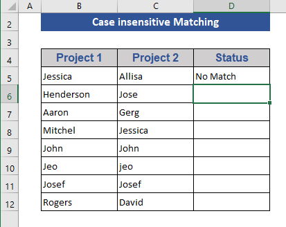
Step 2:

• Then, press Enter.

Step 3:

• Pull the Fill Handle icon.

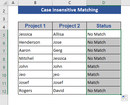
Now, in the status column, we see that Match where both columns are the same otherwise No Match.

1.2 Case-sensitive Approach

The EXACT function compares two text strings and returns TRUE if they are the same, otherwise shows FALSE. EXACT is case-sensitive but ignores formatting differences.

Syntax:

EXACT(text1, text2)

Arguments:

text1 – It is the first text string.

text2 – It is the second text string.

Here, we will use the Exact Function. Which gives a match result with case sensitivity.

Step 1:

• Go to Cell D5 like previously.
• Modify the IF function and EXACT function with this. So, the formula is:

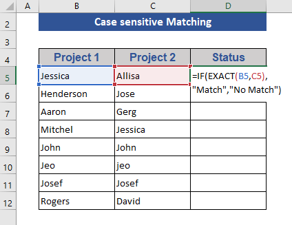
Step 2:

• Press the Enter button.

Step 3:

• Drag the Fill Handle icon.

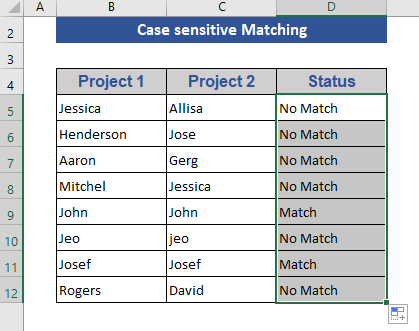
Here, we see that No Match is showing in the 10th row, because of case sensitivity.

Read More: Excel formula to compare two columns and return a value

2. Merging Excel IF, ISNA and MATCH Functions to Return Mismatched Items from 2nd Column

The MATCH function is used to find any matched object. If it finds any match then returns the position from the text or text series.

Syntax:

MATCH(lookup_value, lookup_array, [match_type])

Arguments:

lookup_value – This object will be searched in the lookup_array. It may be any text, numeric value, etc.

lookup_array – This is our range where we will search for lookup_value.

match_type – It is optional. It defines the type of matching.

The ISNA function is a version of the IS functions.

Syntax:

ISNA(value)

Argument:

value – Value refers to the #N/A (value not available) error value.

Step 1:

• First, go to Cell D5.
• Then, write down the formula. The formula is:

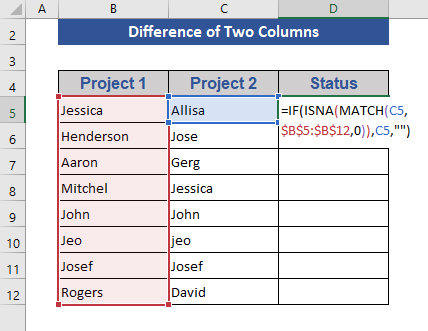
Step 2:

• Now, press Enter.

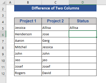
Step 3:

• Pull the Fill Handle icon till the last cell with data.

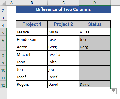
In the status box, we see those names that are present only in Project 2 not in Project 1.

3. Inserting Formula with VLOOKUP Function to Compare and Return Value from Two Columns

The VLOOKUP function is used when we need to find things in a table or a range regarding rows. In VLOOKUP we need to arrange data in a way so that it can check data towards the left. And provides a result after checking.

Syntax:

VLOOKUP (lookup_value, table_array, col_index_num, [range_lookup])

Argument:

lookup_value – This value will be checked. It stays in the initial column of the data range.

table_array – This is the range from where we will search the lookup_value.

col_index_num – This number defines from which column we need the return value.

range_lookup – This is optional. This argument defines the type of matching. It can be exact matching or approximate matching.

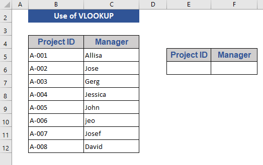
In this section, we will use the VLOOKUP function. Before that, we need to modify our data. After modification data will look like this.

Step 1:

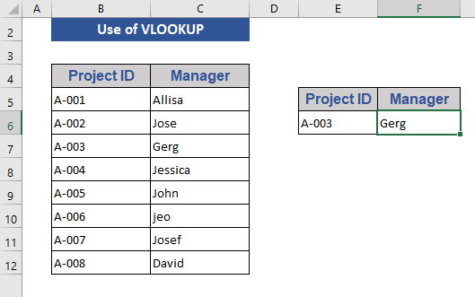
• In the data set, we add two boxes for Project ID and Manager. We will input the Project ID and get Manager’s name instantly.

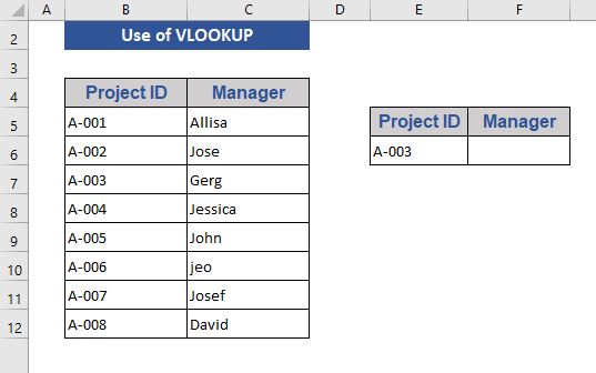
Step 2:

• We put Project ID A-003.

Step 3:

• Go to Cell F6.
• Write the VLOOKUP So, the formula is:

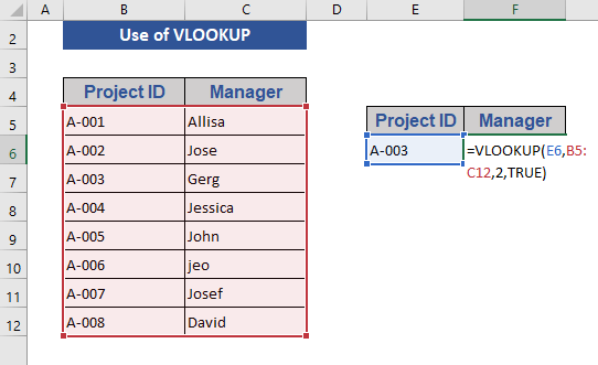
Step 4:

• Then press Enter.

We get the Manager’s name by inputting the Project ID.

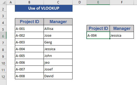
Step 5:

We change the Project ID and press Enter to see the changes.

4. Joining INDEX and MATCH Functions to Compare Two Columns and Return Value

The IFERROR function is used to check errors. It can easily find any error after evaluating a value. If no error is found then give a proper value of the function.

Syntax:

IFERROR(value, value_if_error)

Arguments:

value – The given weight will be used to check to find the error.

value_if_error – This value will be shown if any error is found.

The INDEX function is used in two ways. If we want to return the value of a specified cell or array of cells, see Array form. Or see the reference form If we want to return a reference to specified cells.

Syntax:

INDEX(array, row_num, [column_num])

Arguments:

array – It is the range of cells or an array constant.

row_num –  It is required unless column_num is present. It selects the row in an array from which to return a value. If row_num is omitted, column_num is required.

column_num – It elects the column in the array from which to return a value. If column_num is omitted, row_num is required.

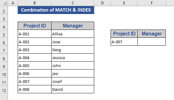
Step 1:

• We took A-007 as the Project ID in Cell E6.

Step 2:

• Write the combination of INDEX and MATCH The formula will be:

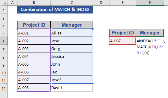
Step 3:

• Then press Enter.

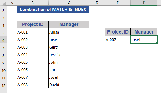
We get the manager’s name according to the project ID. If we give any input on the Project id box that is not present on our data set see what happens.

Step 4:

• We give an input A-010 and press Enter.

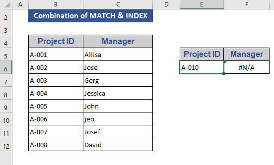
The result is showing #N/A. To avoid those values we will insert the IFERROR function.

Step 5:

• Add the IFERROR function with the existing formula. So, the formula will be:

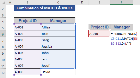
Step 6:

• Then, press Enter.

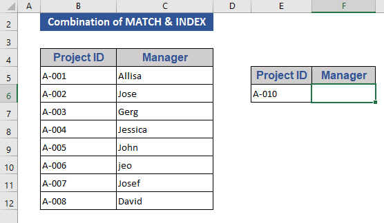
Now, due to using the IFERROR function if the reference is not found on the data the result will be blank.

Formula Breakdown:

• MATCH(E6,B5:B12,0)

This function searches for a match of Cell E6 in the range B5 to B12.

Output: 7

• INDEX(C5:C11,MATCH(E6,B5:B12,0))

This function searches the output of the MATCH function on the range C5 to C11.

Output: Josef

• IFERROR(INDEX(C5:C11,MATCH(E6,B5:B12,0)),””)

This will return the value of INDEX if the value is valid, otherwise, the cell will show blank.

Output: Josef

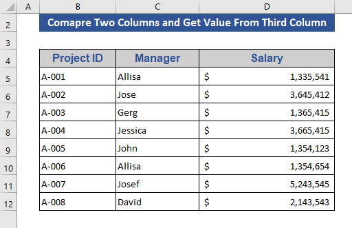
5. Comparing Two Columns and Return Value from Third Column

In this section, we will compare two columns and get results from the third column. We modify the data set first.

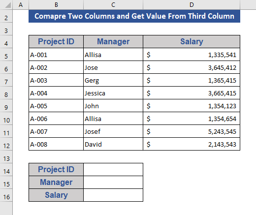
Step 1:

• We will use Project ID and Manager as references to compare and get the output from Salary.

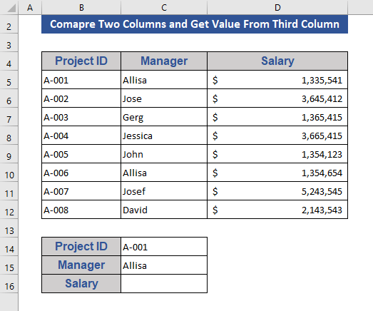
Step 2:

• Give input on the reference boxes.

Step 3:

• Now, write the formula in Cell C16. The formula is:

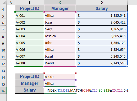
Step 4:

• Then, press Ctrl+Shift+Enter as it is an array function.

Now, we see that the result is from the third column.

Download Practice Workbook

Conclusion 

In this article, we showed an Excel formula to compare two columns and return a value. I hope this will satisfy your needs. Please give your suggestions in the comment box if you have any. Goodbye!

<< Go Back to Columns | Compare | Learn Excel