Filtering data based on cell values in Excel is a process that allows you to display only the rows that meet specific criteria or conditions set by users.
In this Excel tutorial, you will learn how to filter data based on cell value in Excel using 4 useful methods with some practical examples and cases.
Have a look at the following GIF, it shows the filtered rows based on the device name from the drop-down selection.
Filtering data based on cell value can be performed using several methods like keyboard shortcut, Filter command, FILTER function, and VBA. We covered some practical examples and cases to give you a better understanding.
1. Apply Keyboard Shortcut to Filter Data Based on Cell Value
In our very first method, you will learn a keyboard shortcut to filter data based on a cell value in Excel. It’s a very fast approach that will save you time when you want to filter your data based on a cell value in your dataset.
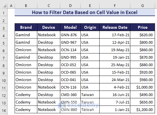
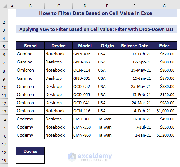
But before that, get introduced to our dataset that contains some companies’ devices, model names, origins, release dates, and corresponding prices.
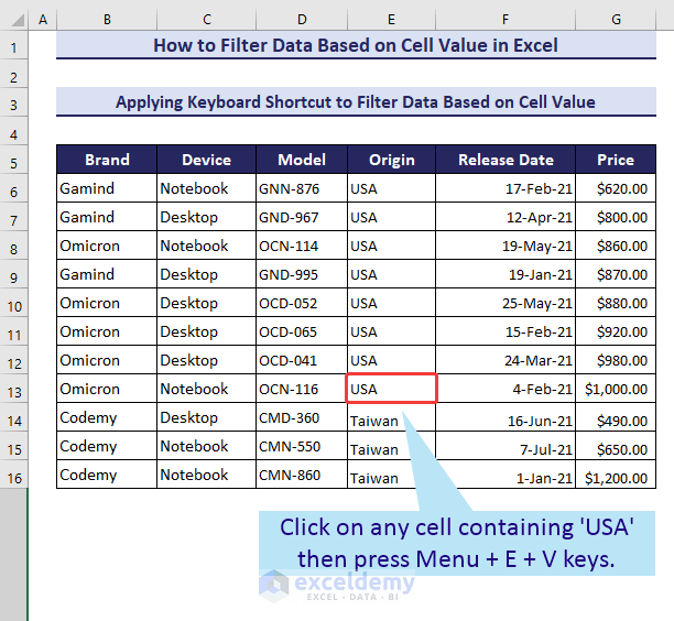
- First, select a cell for which value you want to filter your dataset. Here, we’ll filter for origin ‘USA’.
- Then, press and hold the Menu key on your keyboard and press E + V.
- Instantly, the Filter command will be activated and it will show the filtered rows based on your selection.
2. Filter Data Based on Cell Value by Using Filter Command
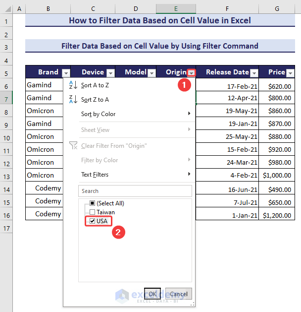
Now, we’ll use the Filter command from the Home tab in this method to filter our data based on the ‘USA’ origin.
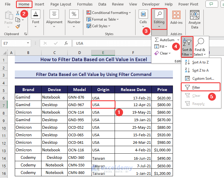
- Select any cell of your dataset.
- Then click as follows: Home >> Editing >> Sort & Filter >> Filter.
- Soon after, the Sort & Filter icon will be visible in every header of your dataset.
- Click on the Sort & Filter icon of the ‘Origin’ header and mark ‘USA’ from the list.
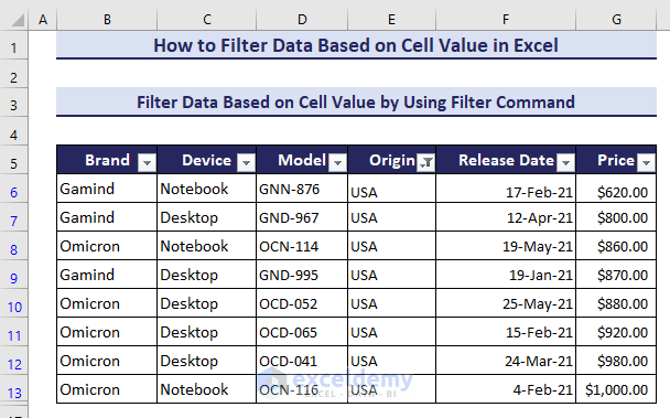
Here’s the filtered result.
3. Apply FILTER Function to Filter Data Based on Cell Value
In this section, we’ll use the FILTER function to filter data based on cell values in Excel. We’ll cover 6 different types of examples so that you can easily understand the uses of it.
Example 1: Filter for a Range
In this example, we’ll apply the FILTER function to filter the data based on a price range- $700 to $1000.
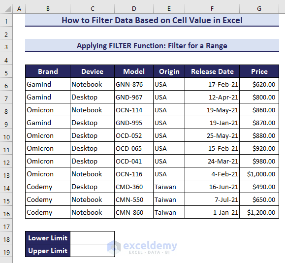
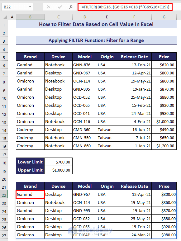
- Insert the following formula in cell B22 and hit the Enter button-
=FILTER(B6:G16, (G6:G16 >C18 )*(G6:G16<C19))The formula will return the filtered result as an array like the image below.
If you change the range values, it will instantly update the filter result as shown below.
Example 2: Filter for Specific Text
Here, we’ll use the IFERROR, ISNUMBER, and SEARCH functions with the FILTER function to filter the data for specific text. The SEARCH function can search text for partial or exact matches, so we’ll be able to filter our data for any partial text. Let’s filter the data for the model name that has the term ‘ocd’.
- Apply the following formula in cell B21 and press the Enter button-
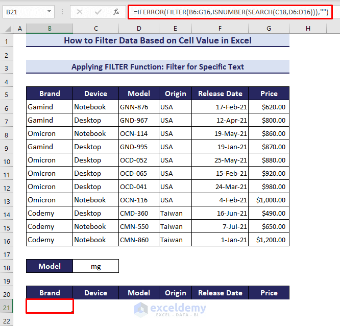
=IFERROR(FILTER(B6:G16,ISNUMBER(SEARCH(C18,D6:D16))),"")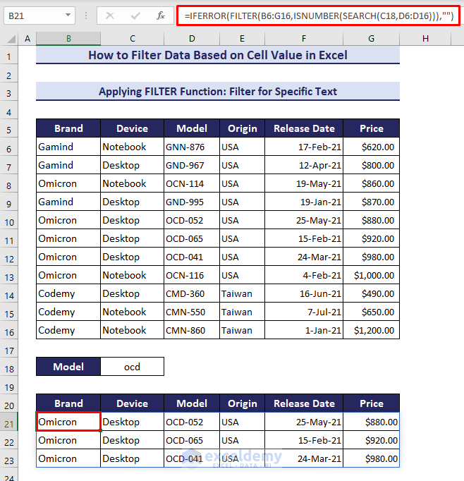
Here’s a GIF image to give the approach a better view. Whenever you type a text partially, it will return the matched result.
- If there happens no match with the criteria, we use the IFERROR function to avoid #CALC! It will return empty instead of #CALC! Error.
Example 3: Filter Data Based on Date
In this example, we’ll use the FILTER function to filter our dataset for a specific date.
- Use the following formula in cell B21 to filter the data for the date 19-May-21:
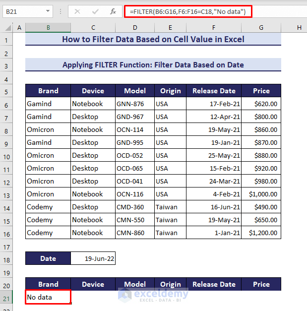
=FILTER(B6:G16,F6:F16=C18,"No data")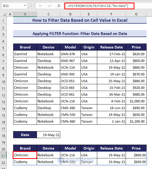
- If the date doesn’t match with any date of our dataset, the FILTER function will return “No Data”.
Example 4: Dynamic Filter with Drop-Down List
In example 2, we used the SEARCH function with the FILTER function to filter data based on cell value with partial match. Here we’ll use the SEARCH function for complete text with a dynamic drop-down list created by the Data Validation tool.
- Insert the following formula in cell B21 to filter the data for ‘Desktop’-
=FILTER(B6:G16,ISNUMBER(SEARCH(C18,C6:C16)))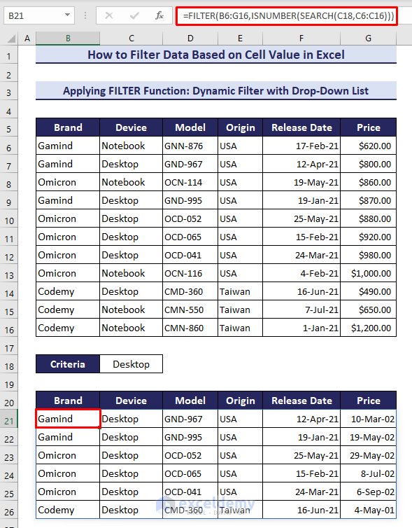
- Then we created a drop-down list by using the Data Validation tool to get the result in a dynamic way.
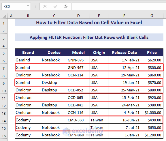
Example 5: Filter Out Rows with Blank Cells
Here, we’ll filter out the rows from our dataset that contain blank cells. For that, we modified our dataset by keeping some blank cells in some rows as shown in the image below.
- Now insert the following formula in cell B19 and press Enter to filter out the rows with blank cells:
=FILTER(B6:G16,(C6:C16<>"")*(D6:D16<>""),"No Result")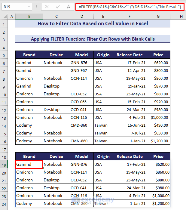
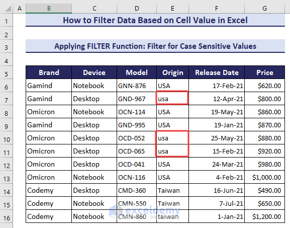
Example 6: Filter for Case Sensitive Values
Now, we’ll use the EXACT function with the FILTER function to filter data by matching the exact case. Because the EXACT function is used to check if two or more than two text strings or values are exactly equal.
Have a look at our modified dataset, in the Origin column, there are two types of cases for the same origin- ‘USA’ and ‘usa’.
- Apply the following formula in cell B21 to filter the data for ‘usa’-
=FILTER(B6:G16,EXACT(E6:E16,C18))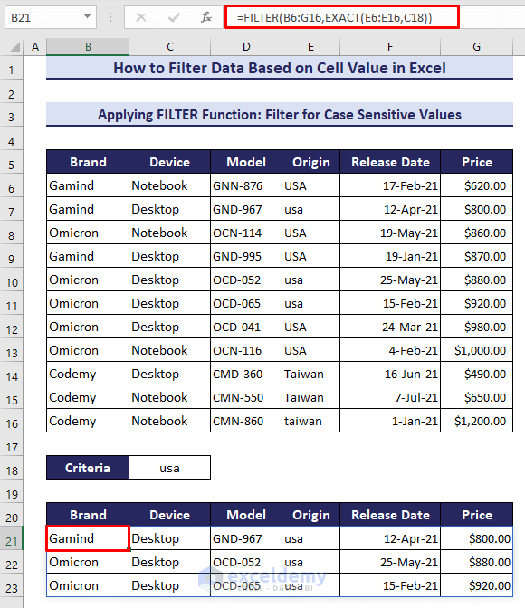
Here’s a better view, according to your typed case, the formula will return the result.
4. VBA Code to Filter Data Based on Cell Value
In our last method, we’ll use VBA to filter based on cell value. We’ll show two useful cases.
Case 1: Filter for Top N Values
First, we’ll apply a VBA code to filter the data for top N values from the Price column.
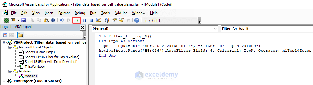
- Insert the following code after opening a new module-
Sub Filter_for_top_N()
Dim TopN As Variant
TopN = InputBox("Insert the value of N", "Filter for Top N Values")
ActiveSheet.Range("B5:G16").AutoFilter Field:=6, Criteria1:=TopN, Operator:=xlTop10Items
End Sub- Then run the code by clicking on the Run icon or by pressing F5.
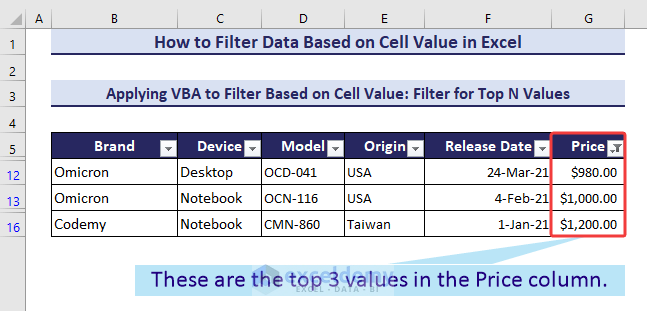
- An input box will open up to insert the value of N. We inserted 3.
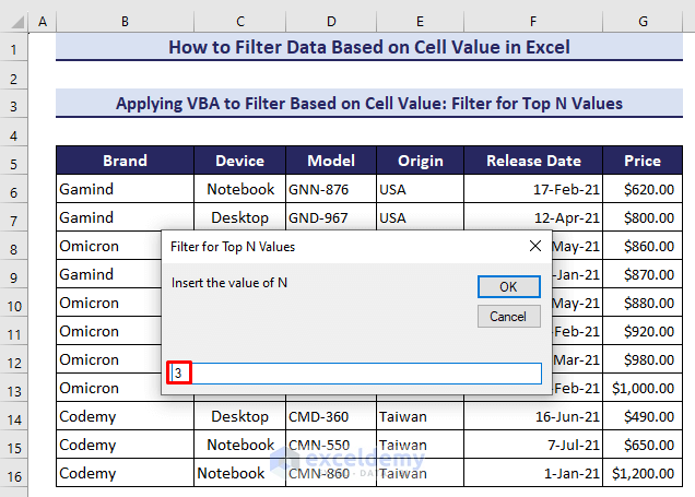
- Soon after, the dataset will be filtered based on the top 3 values of the Price column.
Case 2: Filter with Drop-Down List
Now, we’ll use a VBA code with a drop-down list to filter the data based on the device name. We’ll create the drop-down list in cell B19.
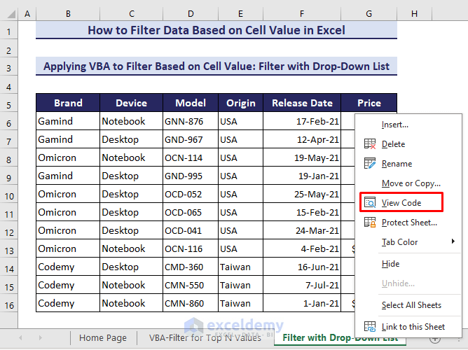
- Remember, We’ll have to keep this code on the sheet, not in the module. For that, right-click your mouse on the sheet name.
- Then select View Code from the context menu.
- Keep the following code in the opened sheet-
Private Sub Worksheet_Change(ByVal Target As Range)
If Target.Address = Range("B19").Address Then
Range("B5:G16").CurrentRegion.AdvancedFilter Action:=xlFilterInPlace, CriteriaRange:=Range("B18:B19")
End If
End Sub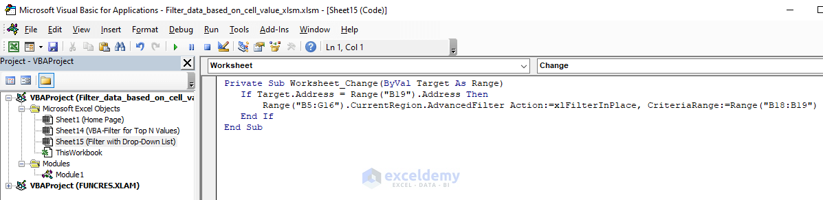
- Now, if we change the value in cell B19, the VBA code will automatically filter the data range according to that value.
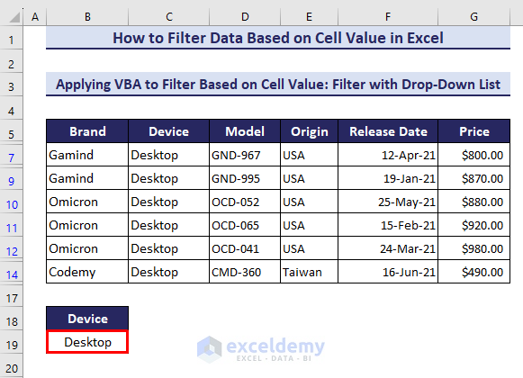
- Finally, we added a drop-down list in cell B19 to filter by using easy selection.
Download Practice Workbook
This article has shown 4 useful methods with some practical examples and cases to filter data based on cell value in Excel. We showed a VBA method and used drop-down lists to perform the filtering operation more dynamically. Filtering data based on cell values is especially valuable while performing data cleaning, identifying and isolating specific data points, and generating customized reports. Thanks for reading and please give your valuable feedback in the comment section.
<< Go Back to Data | Filter in Excel | Learn Excel
Get FREE Advanced Excel Exercises with Solutions!
