How to Apply Conditional Formatting Formula in Excel If Cell Contains Text (6 Practical Cases)

Excel conditional formatting formula if a cell contains text means highlighting those cells that contain any text value or specific text value by applying Excel conditional formatting rules with formula.

In this Excel tutorial, you will learn how to use the Excel formula in conditional formatting to highlight cells containing text values based on certain criteria.

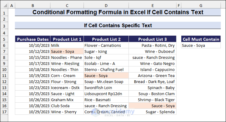
For example, in the GIF below, we have a data set containing three Product Lists along with their Purchasing Dates. Certainly, there are some products in common with each other. In cell G6, we type the product names (e.g., corn, wine, sauce), and the cells containing the product names get highlighted. We have done this by applying a formula to the conditional formatting rule. Go through the full article to learn how we have done it.

Applying the conditional formatting formula to highlight cells if they contain text can be done for various cases. Firstly, we will show you how to highlight any cell with text values in a range. Then, we will apply a conditional formatting formula to highlight the cells to find the exactly matched or partially matched text values.

⏷ Highlight Cells If Cells Contain Text
⏷ Highlight Cells If Cells Contain Specific Text
⏷ Highlight Cells If Cells Contain Case-Sensitive Text
⏷ Highlight Cells If Cells Contain Partial Matched Text
⏷ Highlight Cells If Cells Contain One of Many Text String (OR Logic)
⏷ Highlight Cells If Cells Contain Several Text Strings (AND Logic)

1. Applying Excel Conditional Formatting Formula to Highlight Cells If Cells Contain Text

In this section, we will apply a conditional formatting formula to highlight cells if they contain any text value.

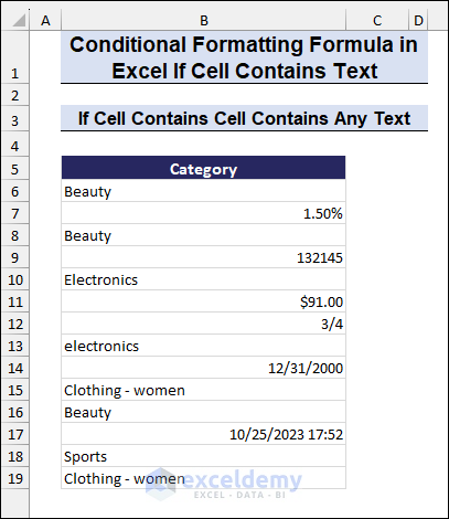
In the image below, you can see a sample data set containing different value types (e.g., text, number, currency, etc.). We will use the formula with the ISTEXT function and apply conditional formatting to highlight the text values only.

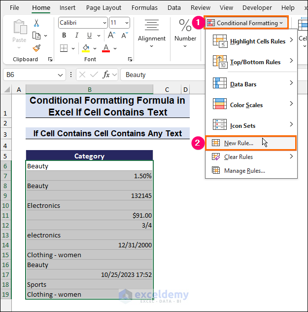
Select the cells to apply conditional formatting.

From the Styles group, click on the Conditional Formatting command.
Select the New Rule command.

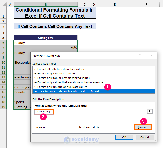
The New Formatting Rule dialog box will appear.
From the Select a New Rule Type list, click on Use a formula to determine which cells to format.
In the Format values where this formula is true box, enter the following formula:

=ISTEXT(B6)

Click on Format to open the Format Cells dialog box.

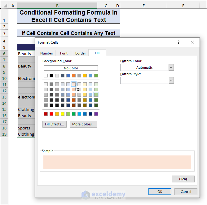
From the Format Cells dialog box, format anything (e.g., number, font, border, fill) as you prefer.
We have selected a fill color, as you can see in the image below.
Click OK.

So, a Format Preview will appear.
Finally, click OK to apply the Conditional Formatting.

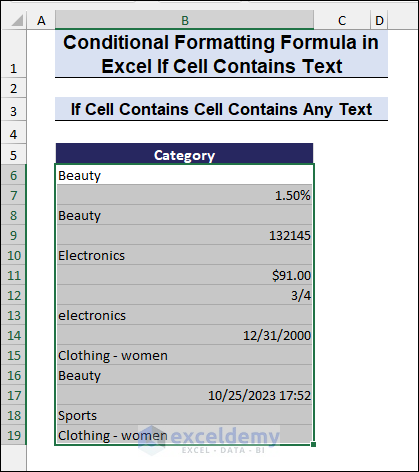
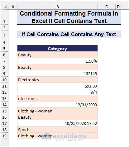
Therefore, we will get the highlighted cells with conditional formatting for containing the text values only.

2. Apply Conditional Formatting Formula to Highlight Cells If Cells Contain Specific Text

In this section, we will apply a conditional formatting formula to highlight cells if they contain the specific text you are looking for. For this purpose, we will use the EXACT function.

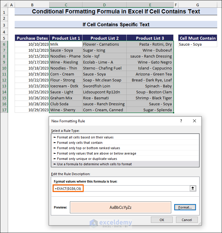
For example, we have the following dataset with three product lists (Product List 1, Product List 2, and Product List 3) along with their purchasing dates. In our product lists, there are some products in common. Here, we want to format the cells that contain exactly the “Sauce – Soya”. In cell G6, we have placed our lookup value. This method will help find duplicates in your dataset.

Repeat the procedures from the previous method to open the New Formatting Rule dialog box.
Then, enter the following formula in the Format values where this formula is true box:

=EXACT($G$6,C6)

Click on Format to apply the formatting as before.

After applying the formatting, we will get the highlighted cells that contain exactly the text “Sauce – Soya”.

3. Using Conditional Formatting Formula to Highlight Cells If Cells Contain Case-Sensitive Text

In this section, we will apply a conditional formatting formula to differentiate the cells containing the case-sensitive text. To do so, we will use the FIND function, which is case-sensitive.

Enter the following formula in the Format values where this formula is true box:

=FIND($G$6,C6)

Click on Format to apply the formatting as before.
After selecting the desired format, click OK to apply.

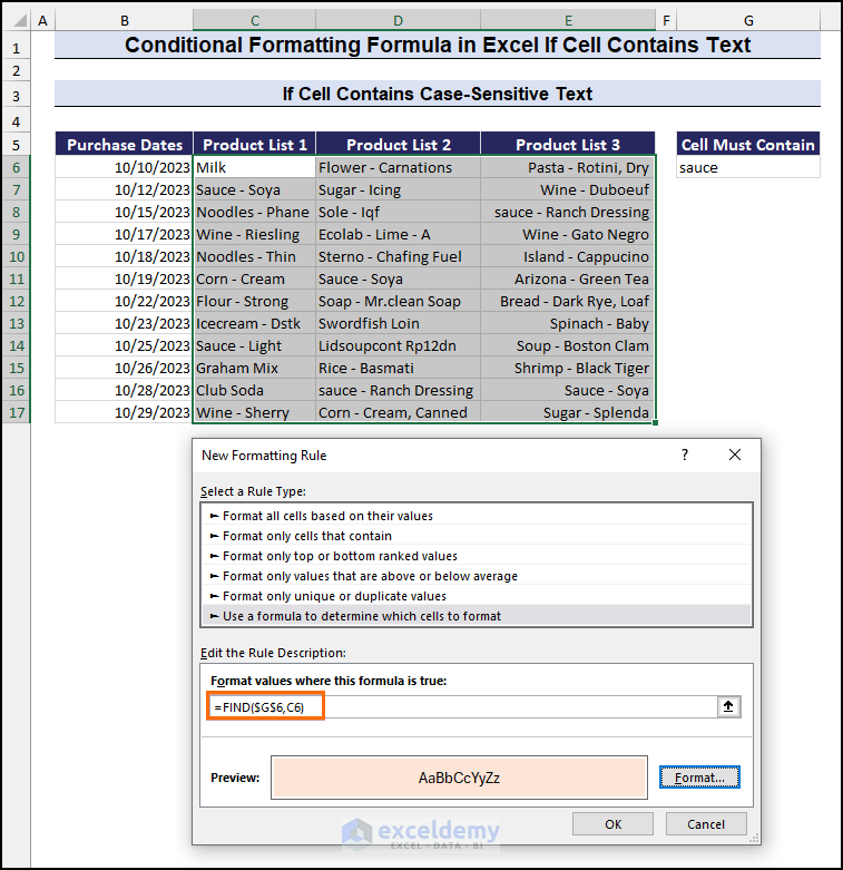
As a result, you can see that the cell formatting changes when you change the value (e.g., Sauce) from upper case to lower case in cell G6.

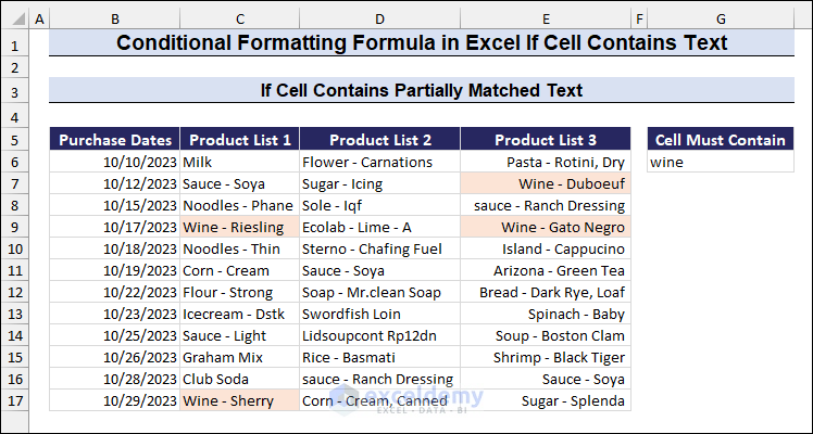
4. Apply Conditional Formatting Formula in Excel to Highlight Cells If Cells Contain Partial Matched Text

In this section, we will apply a conditional formatting formula to highlight the cells if they contain partially matched text. To do that, we will use the SEARCH function.

The benefit of using the SEARCH function is that it is not case-sensitive, and it finds any matches from a cell partially or fully.

For example, we want to highlight the cells containing “wine”. So, we will highlight all the available entries in the wine category.

Enter the following formula in the Format values where this formula is true box:

=SEARCH($G$6,C6)

Click on Format to apply the formatting as before.
After selecting the desired format, click OK to apply.

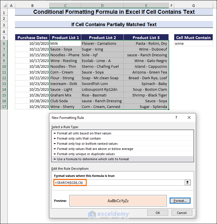
In the image below, we will get the highlighted cells with the formula in conditional formatting for containing the text value (wine) partially.

You can see in the below GIF that the cells are highlighted according to the value in cell G6 (e.g., sauce, corn). It is irrespective of the case, as the SEARCH function is not case-sensitive.

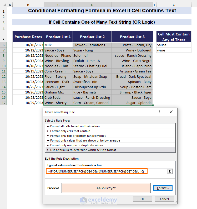
5. Using Conditional Formatting Formula in Excel to Highlight Cells If Cells Contain One of Many Text String (OR Logic)

This section is very useful to describe, as we will apply conditions OR logic. We will highlight the cell values in the range selection that match any of the cell values from cells G6 and G7.

In cells G6 and G7, we will enter the text value Sauce and Wine. So, all the cells will be highlighted that contain any of the cell values of Sauce or Wine.

To do so, we will use a formula combining the IF, OR, ISNUMBER, and SEARCH functions.

Enter the following formula in the Format values where this formula is true box:

=IF(OR(ISNUMBER(SEARCH($G$6,C6)),ISNUMBER(SEARCH($G$7,C6))),1,0)

Click on Format to apply the formatting as before.
After selecting the desired format, click OK to apply.

In the image below, you can see all the highlighted cells that are partially matched with the cell value in cell G6 or cell G7 (Sauce or Wine).

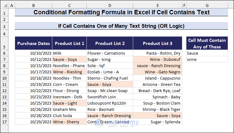
You can see in the below GIF that the cells are highlighted according to the values in cells G6, change the values in G6 and G7, and get all the highlighted values for any of the matches.

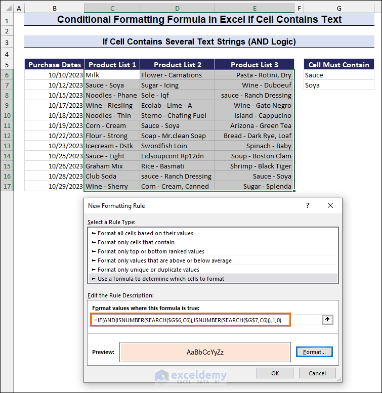
6. Apply Conditional Formatting Formula in Excel to Highlight Cells If Cells Contain Several Text Strings (AND Logic)

Similar to the previous method of applying OR logic, we can also apply a formula in conditional formatting with AND logic. We will highlight the cell values in the range selection that match both the criteria in the cell values G6 and G7.

In cells G6 and G7, we will enter the text values Sauce and Soya. So, all the cells will be highlighted in the selection that contains both the text values of Sauce and Soya.

To do so, we will use a formula combining the IF, AND, ISNUMBER, and SEARCH functions.

Enter the following formula in the Format values where this formula is true box:

=IF(AND(ISNUMBER(SEARCH($G$6,C6)),ISNUMBER(SEARCH($G$7,C6))),1,0)

Click on Format to apply the formatting as before.
After selecting the desired format, click OK to apply.

In the image below, you can see all the highlighted cells that contain both the cell value in cell G6 and cell G7 (Sauce and Wine).

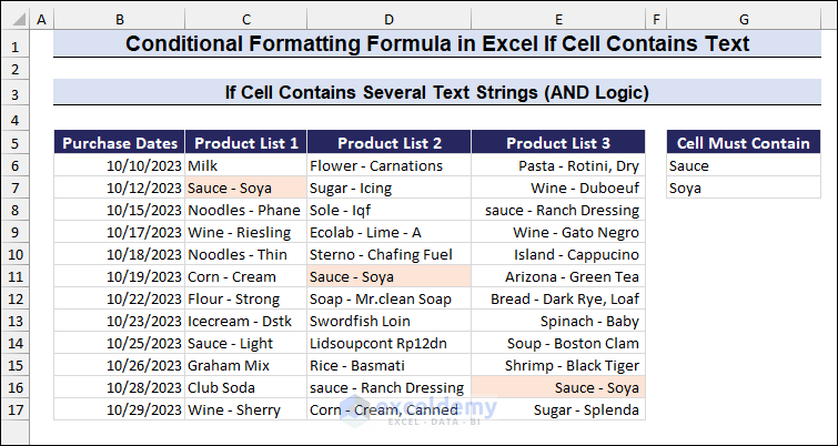
You can see in the below GIF that the cells are highlighted according to the values in cells G6 and G7. Change the values in G6 and G7 and get all the highlighted values for both matches.

Download Practice Workbook

Conditional Formatting Cell Contains Text.xlsx

In this article, we have shown you how to apply the conditional formatting formula in Excel if a cell contains text. You can use these methods to highlight texts with specific criteria, such as case-sensitive text and partial matches. Moreover, you can apply conditional formatting to texts with AND or OR logic. By applying all the methods, you can now easily find your data and make it easy to understand.
Please leave comments in the section below if you have any suggestions or queries. The Exceldemy team always welcomes your valuable feedback.

<< Go Back to Conditional Formatting Formula | Conditional Formatting | Learn Excel

Get FREE Advanced Excel Exercises with Solutions!