Excel Conditional Formatting for Dates Within 30 Days

Conditional formatting has made it easy to highlight important cells or ranges of cells, emphasize unusual values, and visualize data, color scales, and icon sets that related to specific variations in the data. A conditional format changes the outlook of cells based on the conditions that we want. If the conditions return true, the cell range is formatted; if the conditions return false, the cell range is not formatted. It can be used for formatting dates too for any purpose. This article will guide you for conditional formatting dates within 30 days in Excel.

Conditional Formatting for Dates within 30 Days in Excel: 3 Examples

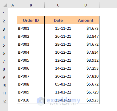
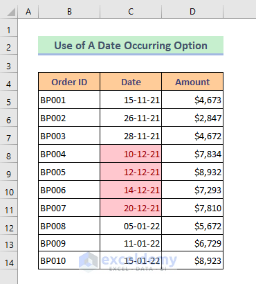
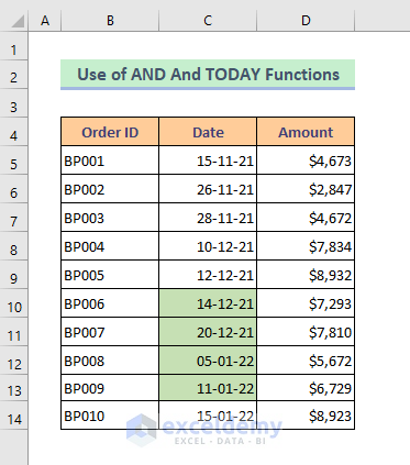
Let’s get introduced to our dataset first. I have placed some order IDs, their order dates, and amounts within 3 columns and 11 rows.

Case 1: Conditional Formatting for Dates within 30 Days for Dates in a Range

In our very first method, I’ll show how to use the Between option of Conditional Formatting to format dates within 30 days. You can set here any date range.

Step 1:

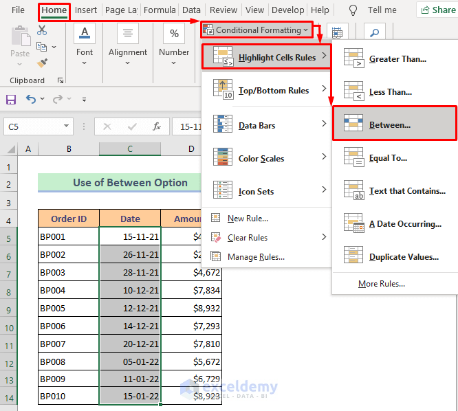
➥ Click as follows: Home > Conditional Formatting > Highlight Cells Rules > Between

A dialog box will open up.

Step 2:

➥ Now set a date range between 30 days. I have set 30-11-21 to 31-12-21.

➥ Press OK then.

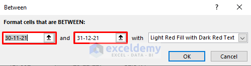
Now we have got our desired dates with highlighted colors.

Read more: Excel Conditional Formatting Based on Date

Case 2: Conditional Formatting for Dates within 30 Days for a Specific Date

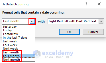
Now we’ll use the A Date Occurring option for conditional formatting dates within 30 days. We won’t need to set dates here, There are some default options here like Last month/ This month/ Next month. We’ll use it directly. But here the limitation is, we can’t use it for the dates before last month or dates after next month.

Step 1:

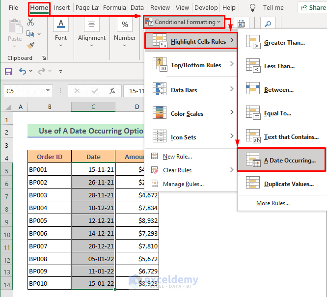
➥ Press as follows: Home > Conditional Formatting > Highlight Cells Rules > A Date Occurring.

A dialog box will appear.

Step 2:

➥ Now select your desired month from the date selection bar.

➥ Then just press OK.

Here’s the output for Last month.

It’s the output for This month.

This last one is the output for Next month.

Read more: Apply Conditional Formatting to Overdue Dates in Excel

Case 3: Combine AND and TODAY Functions with Conditional Formatting for Dates within 30 Days in Excel

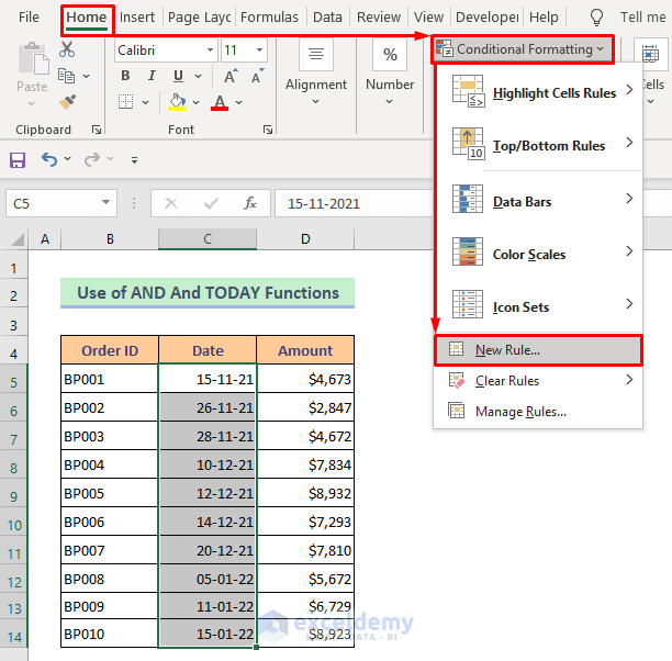
In our last method, I’ll combine the AND function and the TODAY function for conditional formatting dates from today to the next 30 days. The  AND function returns TRUE if all conditions are TRUE and return FALSE if any of the conditions are FALSE. The TODAY function returns the current date.

Step 1:

➥ Click serially: Home > Conditional Formatting > New Rule.

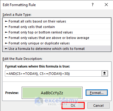
A dialog box named “Edit Formatting Rule” will open up.

Step 2:

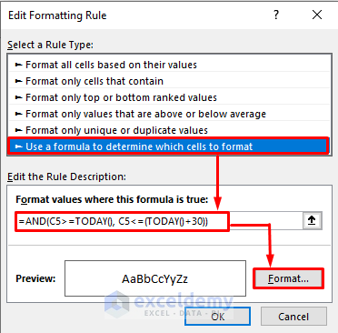
➥ Select Use a formula to determine which cells to format from Select a Rule Type bar.

➥ Then type the formula given below in Edit the Rule Description bar.

➥ Click Format.

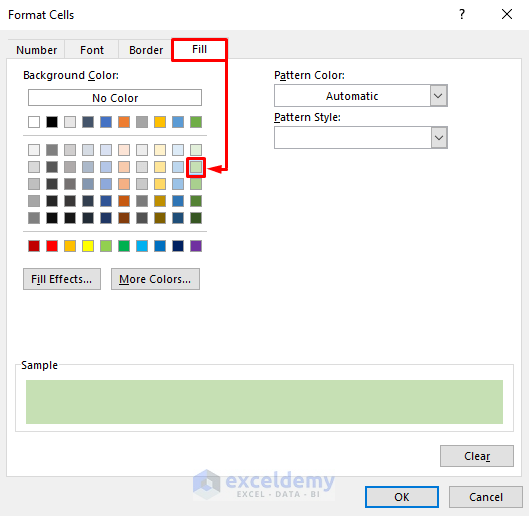
Format Cells dialog box will appear.

Step 3:

➥ Now choose your desired color from the Fill option. I have chosen lite green.

Press OK and we’ll go back to the previous dialog box.

Step 4:

➥ Finally, just press OK.

Now you will observe that the dates from today to the next 30 days are highlighted with our chosen lite green color.

For dates from today to the previous 30 days just apply this formula-

👇 How does the formula work?

➥ C5>=TODAY()

Here, the TODAY function will check if the date in Cell C5 is great than todays’ date or not. So it returns-

FALSE

➥ C5<=(TODAY()+30)

Next, it will check if the date is less than or equal to today’s date + 30 days and returns-

TRUE

➥ AND(C5<=TODAY(), C5>=(TODAY()-30))

Finally, the AND function will encapsulate these two conditions. When both of them are true, the date is highlighted, else it is not highlighted.

Download Practice Book

You can download the free Excel template from here and practice on your own.

Conclusion

I hope all of the methods described above will be good enough for Excel conditional formatting dates within 30 days. Feel free to ask any questions in the comment section and please give me feedback.

Related Articles

• Highlighting Row with Conditional Formatting Based on Date in Excel
• Conditional Formatting Based on Date in Another Cell in Excel
• Apply Conditional Formatting for Dates Older Than Today in Excel
• How to Change Cell Color Based on Date Using Excel Formula
• How to Apply Conditional Formatting to Each Row Individually
• How to Apply Conditional Formatting to Multiple Rows
• How to Highlight Row Using Conditional Formatting
• Conditional Formatting on Multiple Rows Independently in Excel
• How to Change Row Color Based on Text Value in Cell in Excel

<< Go Back to Conditional Formatting Based on Date | Conditional Formatting | Learn Excel