How Do I Create a Pivot Table from Multiple Worksheets (2 Ways)

The article will show you how to consolidate multiple worksheets into one Pivot Table. It is helpful for you to combine or aggregate comparable types of data from multiple worksheets into a single Pivot Table so that you may examine all of the information in those worksheets. An essential tool for conducting an efficient analysis and summarizing the entire dataset is the Pivot Table. In this article, you will see how to create a Pivot Table from multiple worksheets.

How Do I Create a Pivot Table from Multiple Worksheets: 2 Ways

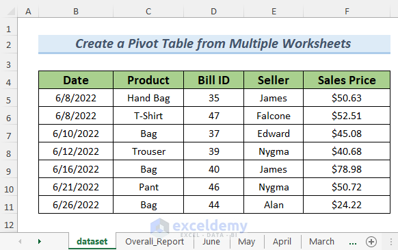
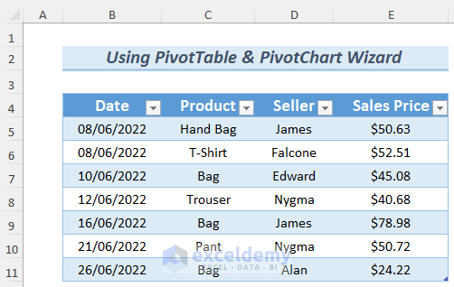
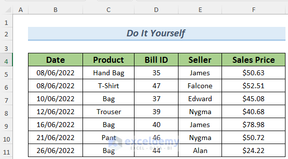
The dataset contains sales statistics on a few products and the vendors who offered them for sale in the months of March, April, May, and June.

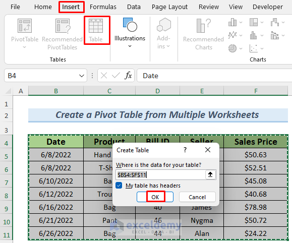
Let’s convert this dataset to a table.

Select the dataset and then go to Insert >> Table.
After that, a dialog box will show up. Make sure you select My table has headers and click OK. You may press CTRL+T to convert the dataset to a table.

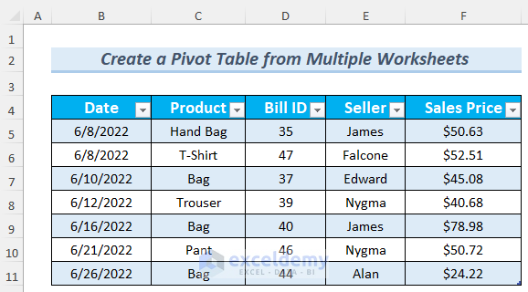
Your data is now transformed into a table. The following sections will make use of our data as tables.

1. Using Power Query Editor to Create a Pivot Table from Multiple Worksheets

Using a Power Query Editor is the most efficient approach to combining multiple worksheets in an Excel Workbook. Let’s go through the procedure below for a detailed description.

Steps:

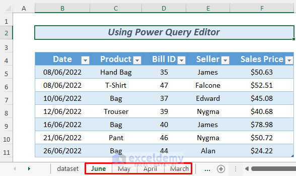
We will be using the following sheets to insert a Pivot Table.

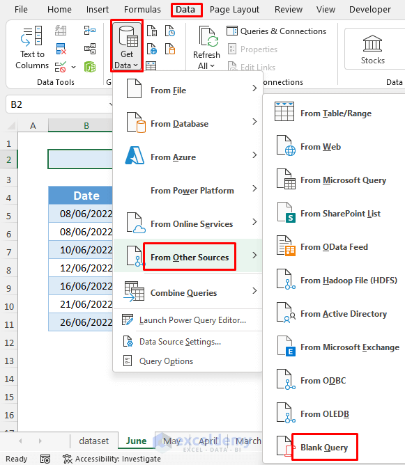
Now, go to Data >> Get Data >> From Other Sources >> Blank Query.

After that, the Power Query Editor will open up.
Next, give your Query a name. In my case, I named my query Overall_Report and hit ENTER.
Later, write down the following formula in the Power Query formula bar and press ENTER.

=Excel.CurrentWorkbook()

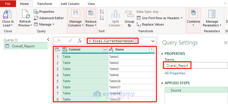
The formula will return all the tables in the workbook.

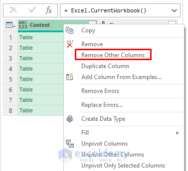
Next, we removed the second column using the Remove Other Columns command from the context menu as we don’t need duplicates, which we can get by right-clicking on the header of the first column.

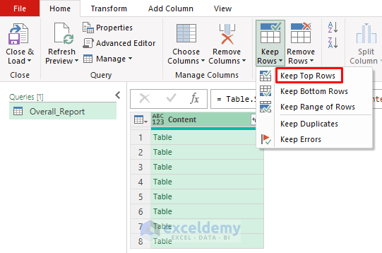
Later, we select Home >> Keep Rows >> Keep Top Rows. We don’t need all the tables in this workbook.

Thereafter, the Keep Top Rows window will appear. As we are working with the first four tables of this workbook, we selected four.

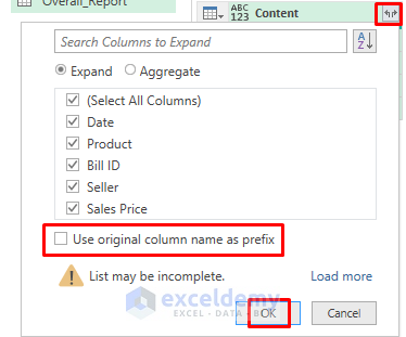
This operation will return the first four rows only. After that, click on the marked icon of the following image, uncheck Use original column name as prefix, and click OK.

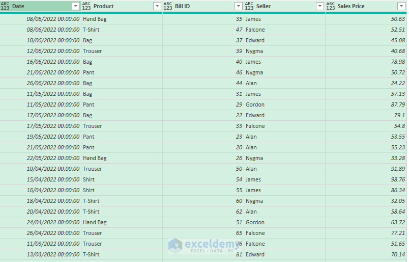
Next, you will see all the data of your sheets consolidated together in the Power Query Editor.

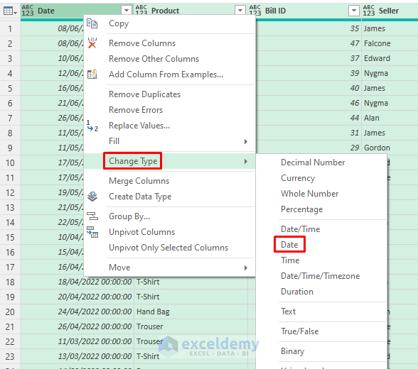
The query contains unnecessary formats like the date and time. When the query opens, you will automatically see that there is a time following every date. To remove this, we clicked right on the mouse while selecting the Date column and then chose Change Type >> Date.

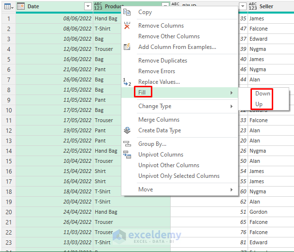
By the way, use the next command if your data contains any blanks. Select the columns that contain blanks and then right-click >> Fill. Select Down or Up according to your convenience.

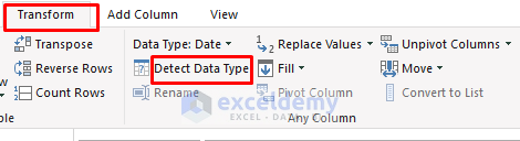
After that, press CTRL+A and then go to Transform >> Detect Data Type. Although it’s not always essential, using this command while using the Power Query Editor is a good habit to get into.

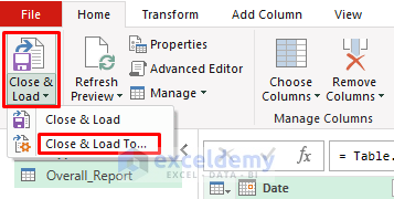
Thereafter, select Home >> Close & Load To…

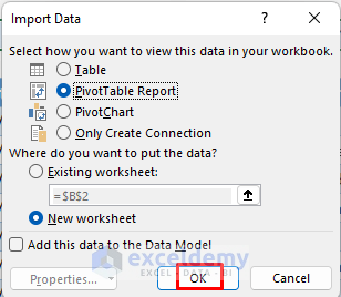
Next, the Import Data dialog box will show up. Select PivotTable Report, the sheet on which you wish to open the Pivot Table, and click OK.

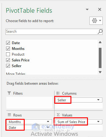
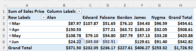
Your Pivot Table will be seen on a new worksheet as we selected a New Worksheet for it. After that, drag the Date range to the Rows Field, Sales Price to the Values Field, and Seller to the Columns Field in order to view the worksheets’ compiled data.

After that, you can view monthly and overall sales reports for the months of March through June. In your Pivot Table, you may also view sales records based on sellers.

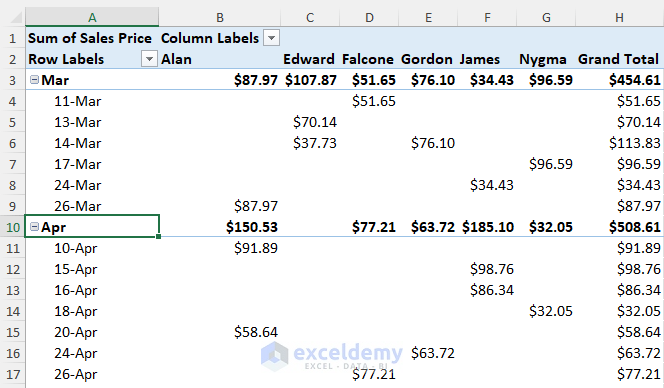
In addition, click on the Plus button next to the month name to see more details about sales in that month. This will return you a date-based sales report.

Thus, you can create a Pivot Table from multiple worksheets by using a Power Query Editor.

2. PivotTable and PivotChart Wizard to Create a Pivot Table from Multiple Worksheets

You can also use the PivotTable and PivotChart Wizard to create a Pivot Table from multiple worksheets of your Workbook. We can still use this method for straightforward sales records even though it has some limitations when it comes to calculating sales. Let’s look at the procedure below.

Steps:

Here, we’ll be using the Sales column. Therefore, we’ll utilize the same worksheets but skip the Bill ID field. The Pivot Table may experience some redundant calculations as a result.

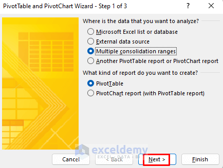
After that, press ALT, D, and P, and you will see the PivotTable and PivotChart Wizard on the screen.
Next, choose the area in which you wish to perform your data analysis. As our article is dedicated to the Pivot Table, we select Multiple consolidation ranges and PivotTable. In addition, If you wish to conduct a thorough analysis, you may select the PivotChart report instead of just PivotTable.
Later, click Next.

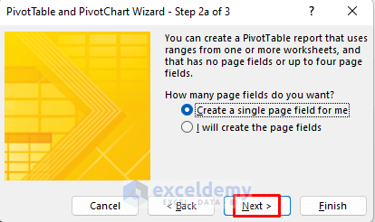
Thereafter, there are two options available for how many page fields you need for analysis. You have the option of creating your own page field or having Excel build one for you automatically. In this case, I select Create a single page field for me, which means Excel will create it automatically for me.
After that, click Next.

Next, a message box will appear on your screen where you can enter the table ranges for the Pivot Table. Simply choose the sheet that contains the report for the table of sales, then choose the table and click Add. First, I selected the table of June (2) sheet.

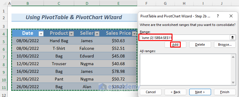
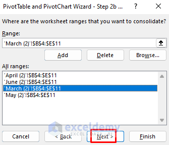
Similarly, add the other tables too.
After that, click Next.

Select New worksheet or Existing worksheet based on your choice.
Click Finish after that.

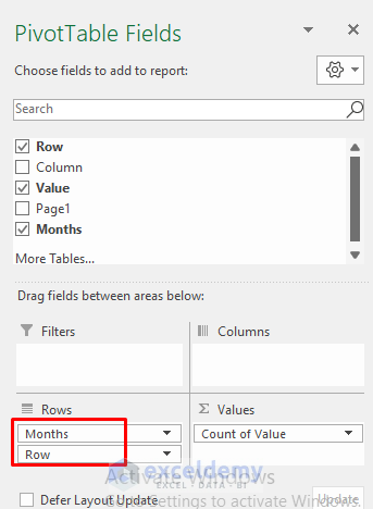
I already said that the first strategy is more effective than this one. We must comprehend the ranges in the PivotTable Fields. Here, Row refers to the dates and Value refers to the sales values. So, drag the Row and Value fields to the Rows and Values fields respectively.

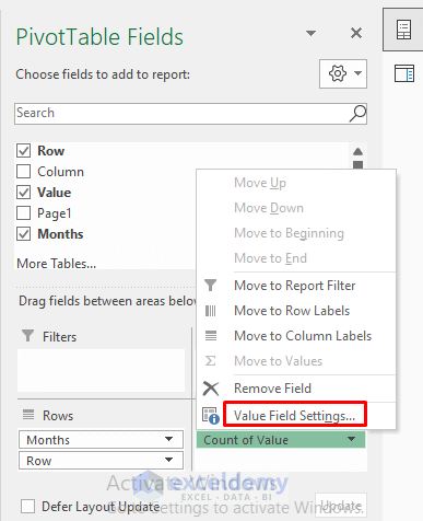
You can observe that the value field of the sales values is in the Count of Value. We need the sales values and their total, so we click on the Count of Value field >> Value Field Settings.

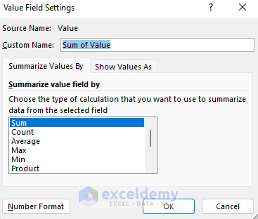
In the Value Field Settings window, we choose Sum of Value and click OK.

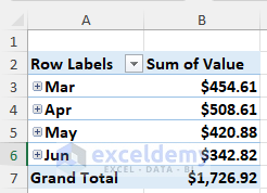
A monthly sales report will be returned by this action in the Pivot Table.

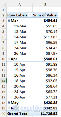
If you wish to daily broaden your analysis, click the Plus icon beside the month name.

Thus, you can create a Pivot Table from multiple worksheets by using the PivotTable and PivotChart Wizard.

Practice Section

Here, I’m giving you the dataset of this article so that you can practice these methods on your own.

Download Practice Workbook

PivotTable from Multiple Worksheets.xlsx

Conclusion

In the end, we can conclude that you can learn the basic ideas of how to create a Pivot Table from multiple worksheets after reading this article. If you have any better methods, questions, or feedback regarding this article, please share them in the comment box. This will help me enrich my upcoming articles.

<< Go Back to How to Create Pivot Table in Excel | Pivot Table in Excel | Learn Excel

Get FREE Advanced Excel Exercises with Solutions!