Dataset Overview
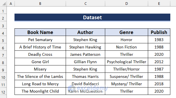
We’ll use the following dataset. It contains several Book Name along with their respective details.
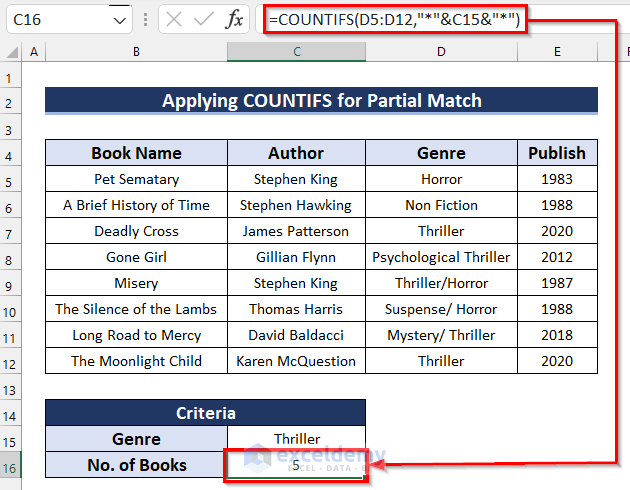
Method 1 – Use the COUNTIF for Partial Matches
- Choose the cell where you want the count of books. For example, let’s select cell C16.
- In cell C16, enter the following formula:
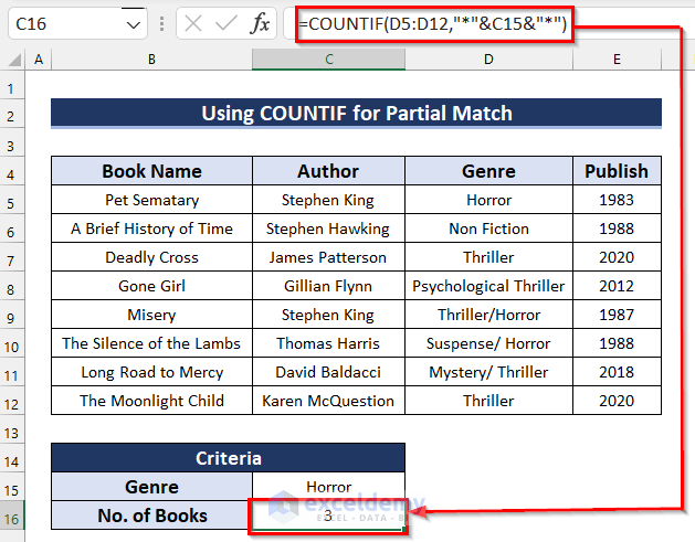
=COUNTIF(D5:D12,"*"&C15&"*")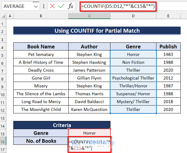
- Press Enter to get the result.
- We use the COUNTIF function with the cell range D5:D12 as the range and “*” & C15 & “*” as the criteria.
- The formula counts the number of cells in the range D5:D12 that partially match the value in cell C15.
Method 2 – Employing COUNTIF for Partial Matches
The COUNTIFS function allows counting based on multiple criteria. Let’s explore two examples:
2.1. Apply COUNTIFS for Partial Matches
- Choose the cell where you want the count of books.
- In the selected cell, enter:
=COUNTIFS(D5:D12,"*"&C15&"*")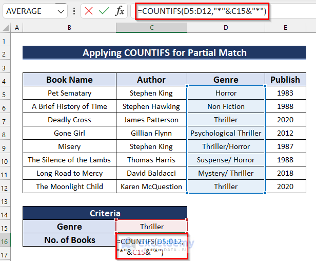
- Press Enter to get the Count of Books.
2.2. Utilizing COUNTIFS for Partial Matches with Multiple Criteria
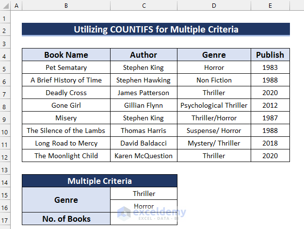
- Choose the cell where you want the Count of Books.
- In the selected cell, enter:
=COUNTIFS(D5:D12,"*"&C15&"*",D5:D12,"*"&C16&"*")
- Press Enter to get the Count of Books.
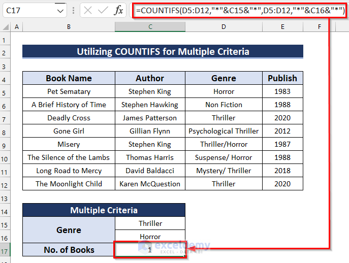
- We use COUNTIFS with two criteria ranges: D5:D12 and the same wildcard pattern for both C15 and C16.
- The formula counts cells that partially match both values.
Method 3 – Using IF and COUNTIF for Genre Comparison
Apart from counting, you can check if a specific genre exists. Here’s how:
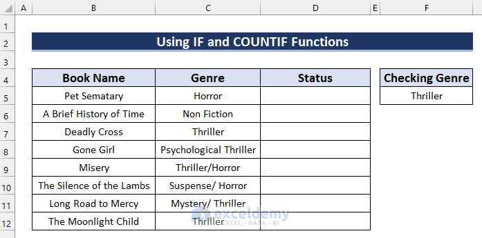
- Choose the cell where you want the status (e.g., cell D5).
- In cell D5, enter:
=IF(COUNTIF(C5,"*"&$F$5&"*"),"Genre Found","Not in search Genre")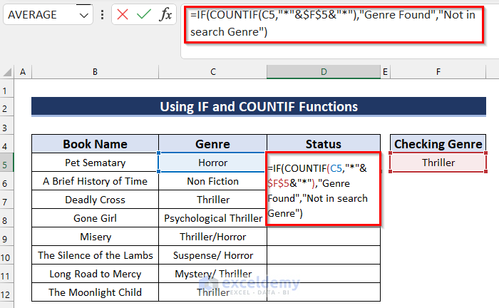
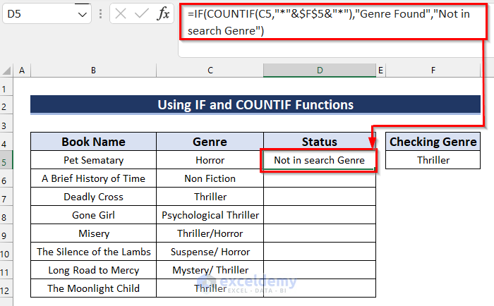
- Press Enter to get the result.
How Does the Formula Work?
- COUNTIF(C5,”*”&$F$5&”*”): counts cells matching the criteria.
- The IF function returns “Genre Found” if true, or Not in search Genre if false.
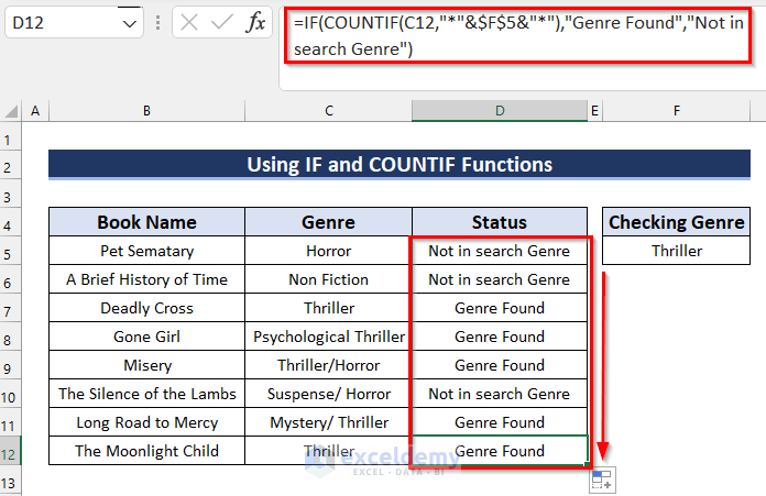
- Drag the Fill Handle down to copy the formula.
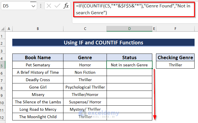
- Below is the desired result:
Alternative to COUNTIF Function for Partial Match in Excel
Instead of using the COUNTIF function, you can use a combination of several functions to achieve the same type of operation. This alternative formula utilizes the SUMPRODUCT function, the ISNUMBER function, and the SEARCH function. Let’s walk through the steps:
- Choose the cell where you want the count of books. For example, let’s select cell C16.
- In cell C16, enter the following formula:
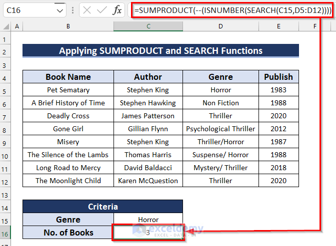
=SUMPRODUCT(--(ISNUMBER(SEARCH(C15,D5:D12))))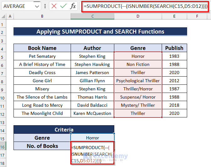
- Press Enter to get the Count of Books.
How Does the Formula Work?
- SEARCH(C15,D5:D12): The SEARCH function looks for the criteria value (C15) within the specified range (D5:D12). It returns the starting position of the search text if found, or an error otherwise.
- ISNUMBER(SEARCH(C15, D5:D12)): The ISNUMBER function checks whether the result of the SEARCH function is a number. It returns a boolean value (True or False).
- –(ISNUMBER(SEARCH(C15, D5:D12))): We use two unary operators (–) to convert the boolean value into 1 or 0.
- SUMPRODUCT(–(ISNUMBER(SEARCH(C15, D5:D12)))): The SUMPRODUCT function processes this array and returns the total sum.
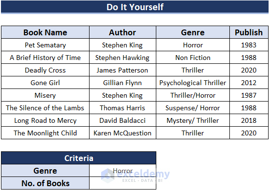
Practice Section
We have provided a practice sheet for you to practice how to use the COUNTIF function for a partial match in Excel.
Download Practice Workbook
You can download the practice workbook from here:
<< Go Back to Partial Match Excel | Formula List | Learn Excel
Get FREE Advanced Excel Exercises with Solutions!
