In Excel, we often work with large datasets. While working with these datasets, we frequently need to combine data from multiple sheets to analyze them properly. In this article, I will explain 4 ways in Excel to combine data from multiple sheets.
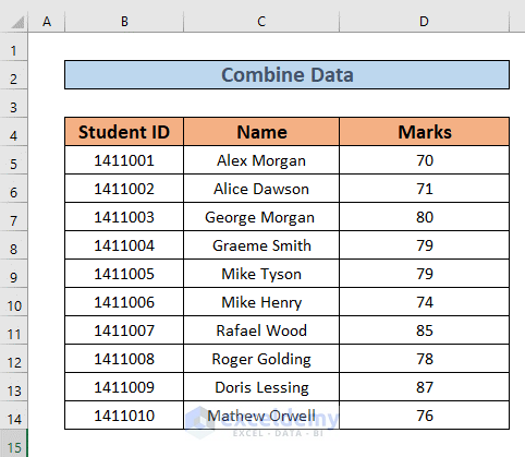
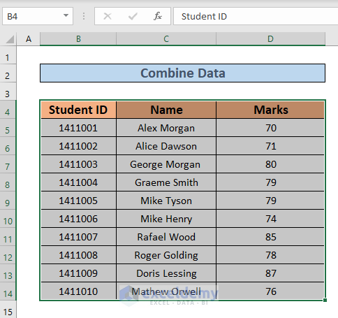
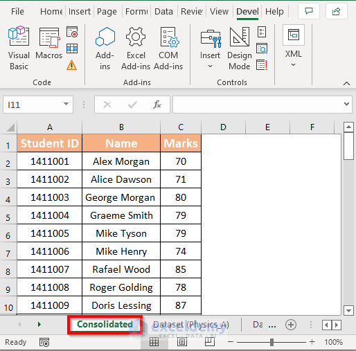
This is the worksheet I am going to use to explain the methods of how to combine data from multiple sheets in Excel. We have several students along with their Student ID and their Marks. I am going to consolidate the Marks for different subjects to describe the methods.
1. Applying Consolidate Feature to Combine Data from Multiple Excel Sheets
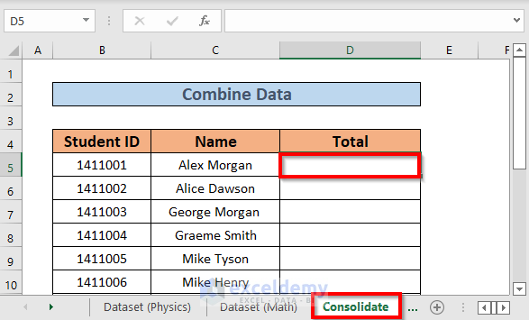
In this section, I will explain how to use the Consolidate Feature to combine data. I will add the Mark(s) of Physics and Math by using this method.
STEPS:
➤ Go to the Consolidate worksheet. Select D5.
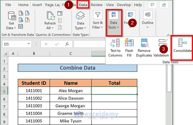
➤ Then go to the Data tab >> select Data Tools >> select Consolidate.
A dialog box of Consolidate will appear.
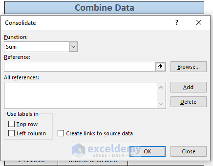
➤ Keep the Function drop-down as it is, since you want to sum the marks.
➤ Now you need to add a Reference. Go to Dataset (Physics) worksheet >> select the range D5:D14 >> select Add.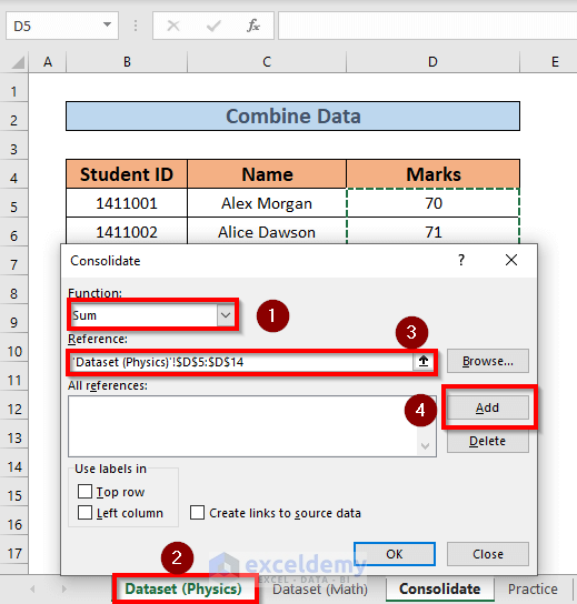
➤ Excel will add the reference. Similarly, set the reference for the range D5:D14 from the Dataset (Math) workbook.
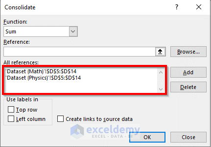
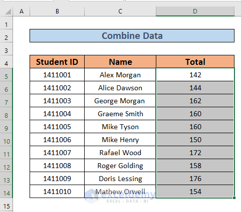
➤ Then click OK. Excel will combine them and return the sum as output.
2. Using Excel Power Query to Combine Data from Multiple Sheets
Now we will see how to combine data from several sheets using Power Query. I will combine the Mark(s) of Physics for two sections (A & B) in this case. There is a prerequisite in this case. The dataset should be in Table form.
STEP-1: CREATING TABLE
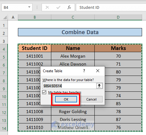
➤ Select the range B4:D14.
➤ Press CTRL + T. Create Table dialog box will pop up. Click OK.
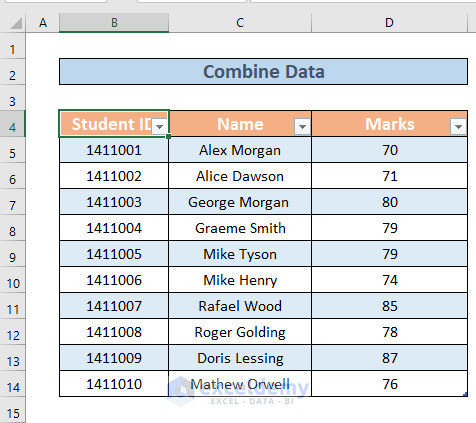
Excel will create the table.
➤ Now I will rename the table. To do so, go to the Table Design tab and rename your table.
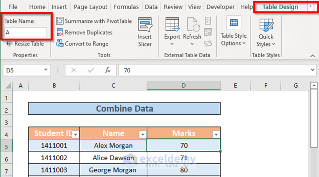
Similarly, create tables for other datasets.
STEP-2: COMBINE DATA
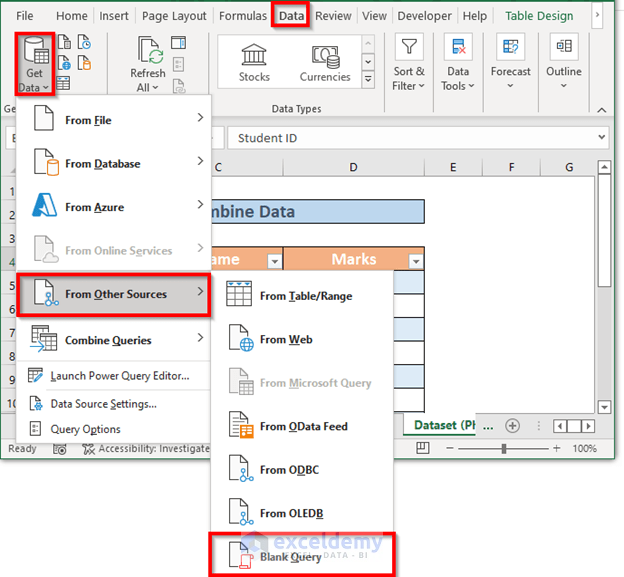
➤ Go to the Data tab >> select Get Data >> select From Other Sources >> select Blank Query
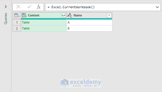
The Power Query Editor window will appear. In the formula bar, write down the formula:
=Excel.CurrentWorkbook() 
➤ Press ENTER. Excel will show the tables in your workbook.
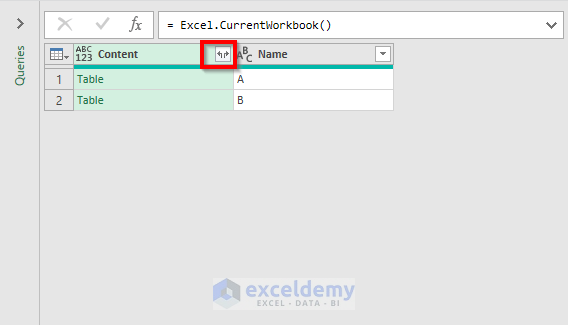
➤ Then, click the double-headed arrow (see image).
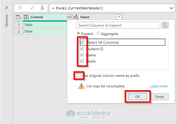
➤ Next, select the columns that you want to combine. I will combine all of them.
➤ Leave the Use original column name as prefix unmarked. Then click OK.
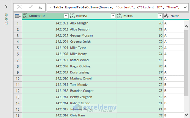
Excel will combine the datasets.
➤ Now, select Close & Load.
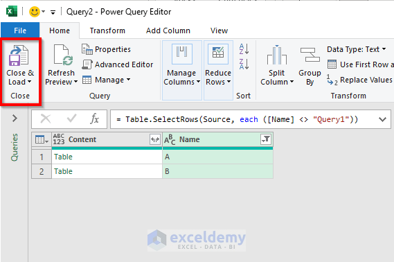
Excel will create a new table combining the datasets.

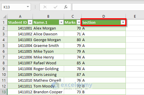
➤ Rename the Name column. I am going to call this Section.
NOTE:
When you use the above method, you may face a problem.
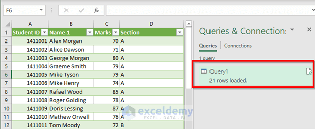
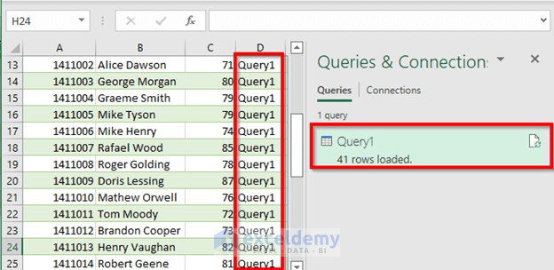
Our new table’s name is Query1 which consists of 21 rows including the headers.
➤ Now right-click your mouse to bring up the Context Menu. Then click Refresh.
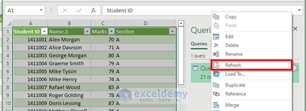
Once you refresh, you will see that the row number has changed to 41. That’s because Query1 itself is a table and is working as input.
To solve this issue, follow the steps.
➤ Go to the drop-down of the column Name (see image)
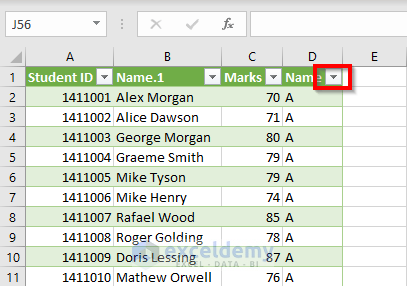
➤ Then go to Text Filters >> select Does Not Contain.
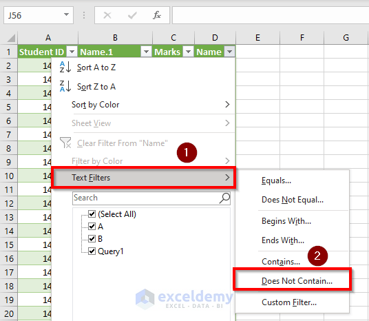
A Custom AutoFilter window will open.
➤ Write Query1 in the box (see image). Then click OK.
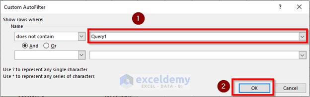
This time, the rows having the name Query1 will not be seen even if you refresh the dataset.
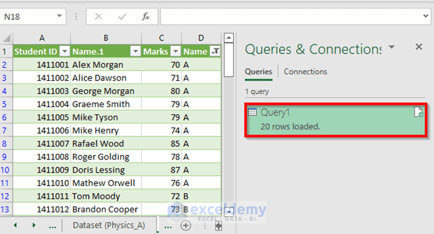
20 rows are loaded now because Excel is not counting the header this time.
3. Combining Data from Multiple Sheets Using VBA Macro Tool
Now I will apply VBA macro to combine data from multiple sheets. Suppose your workbook has two worksheets, Dataset (Physics_A) and Dataset (Physics_B) and you are going to combine the data from these datasets into a new worksheet named Consolidate.
STEPS:
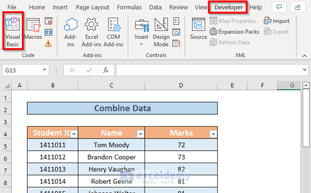
➤ Go to Developer tab >> select Visual Basic.
➤ Then go to Insert tab >> Module.
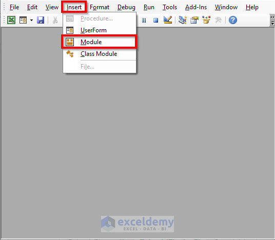
A Module window will appear. Now write the following code.
Sub combine_multiple_sheets()

Dim Row_1, Col_1, Row_last, Column_last As Long
Dim headers As Range

Set wX = Worksheets("Consolidated")
Set WB = ThisWorkbook
Set headers = Application.InputBox("Choose the Headers", Type:=8)
headers.Copy wX.Range("A1")

Row_1 = headers.Row + 1
Col_1 = headers.Column
Debug.Print Row_1, Col_1

For Each ws In WB.Worksheets

If ws.Name <> "Consolidated" Then
ws.Activate
Row_last = Cells(Rows.Count, Col_1).End(xlUp).Row
Column_last = Cells(Row_1, Columns.Count).End(xlToLeft).Column
Range(Cells(Row_1, Col_1), Cells(Row_last, Column_last)).Copy _
wX.Range("A" & wX.Cells(Rows.Count, 1).End(xlUp).Row + 1)
End If

Next ws
Worksheets("Consolidated").Activate

End Sub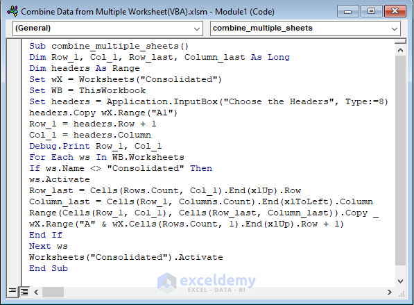
Here, I have created a Sub Procedure named combine_multiple_sheets. I have taken Row_1, Col_1, Row_last, and Column_last variables using the Dim statement and set wX as the Consolidated worksheet using the Set statement.
Also, I used an input message box using Application.InputBox with the statement “Choose the Headers”.
Then, I applied a For loop and defined Row_1 and Col_1 using headers.range property.
➤ Then press F5 to run the program. Excel will create a combined dataset.
NOTE:
Please remember that this VBA code will combine all the sheets available in your workbook. So you must have only those worksheets whose data you are going to combine.
4. Inserting Excel VLOOKUP Function to Combine Data from Multiple Sheets
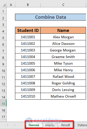
Suppose, I have a worksheet named “Names” where I have the names of some students and another one named “Marks”. To create a proper Result sheet, I need to combine them. I will do that using the VLOOKUP function.
STEPS:
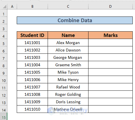
➤ Create a new column, Marks to the right of Names.
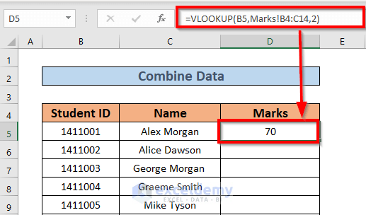
➤ Then, go to D5 and write down the following formula
=VLOOKUP(B5,Marks!B4:C14,2)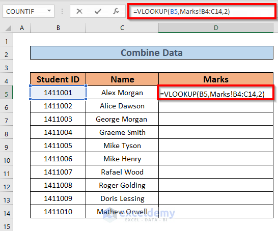
Here, I have set the lookup value to B5 and the array is B4:C14 from the Marks sheet. The col_ind_num is 2 as I want the marks.
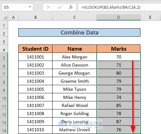
➤ Now press ENTER. Excel will return the output.
➤ Then use Fill Handle to AutoFill up to D14. Excel will combine the marks from the Marks worksheet.
Download Practice Workbook
Conclusion
In this article, I have illustrated 4 ways in Excel to combine data from multiple sheets. I hope this will benefit you. Lastly, if you have any kind of suggestions, ideas, or feedback, please feel free to comment below.
<< Go Back To Merge Sheets in Excel | Merge in Excel | Learn Excel
Get FREE Advanced Excel Exercises with Solutions!
