When you are using Pivot Tables, you can use calculated fields as a way of making your own custom calculations. In this article, we shall learn different techniques of Excel pivot table calculated field.
Pivot Table Reports already provide a set of summary calculations and function options, but sometimes this is not enough for the unique needs that you may have. So, you can add your own needed custom-made formulas using the original fields in the Pivot Table, and have the results of your formulas or calculated fields appear in the Pivot Table.
What do I mean by this? Well, let’s start with a simple example to master the basics of creating calculated fields, and then we can build up from there in follow-up posts.
How to Insert Calculated Field in Pivot table?
A hypothetical biorefinery has a number of different bioreactors on site, producing both biofuel and value-added chemicals. The biorefinery is using microorganisms and the fermentation route in order to produce the desired outputs.
Read More: How to Create Pivot Table Data Model in Excel 2013
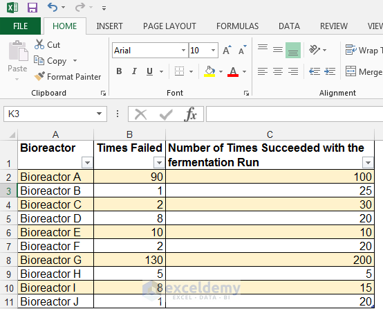
The technicians record the number of times the equipment failed, and the number of times the fermentation runs succeeded. We will show the failure rate of these bioreactors using a calculated field. The reason we would want to show something like the failure rate is, our procurement manager wants to know which equipment suppliers to order bioreactors from, in future, and he wants to see which of the bioreactors on the site were the most reliable.
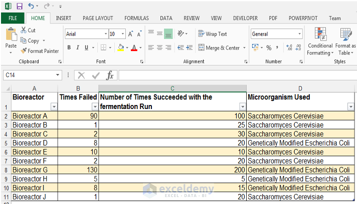
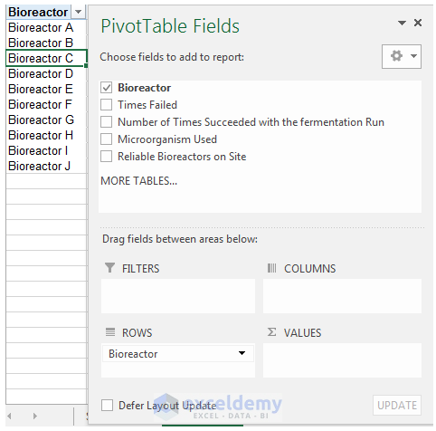
A picture of the source data is shown below:
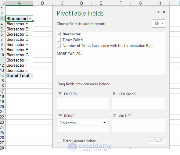
Firstly, you should have your Pivot Table already set up. If you are unsure of how to do this, please visit this post on creating pivot tables in a few easy steps.
Make a simple calculate field
Now let’s get to the fun part.
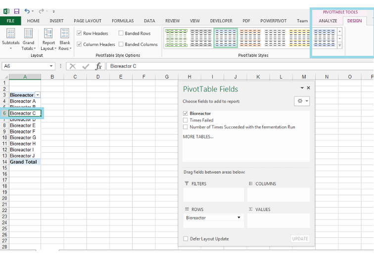
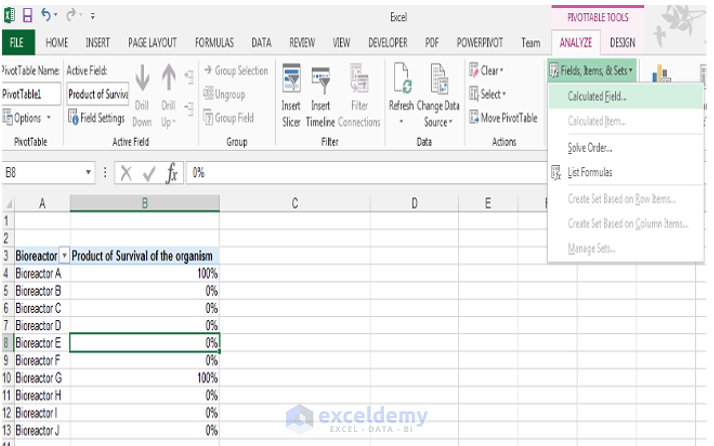
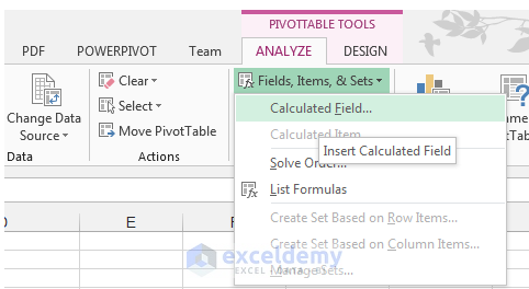
1) With a cell in the Pivot Table selected, in order to activate the context-sensitive Pivot Table Tools, Analyze tab.
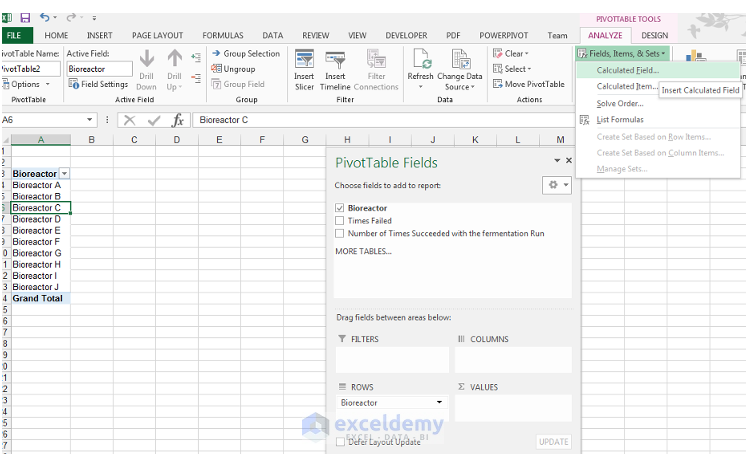
2) Click on the drop-down arrow next to Fields, Items, & Sets in the Calculations Group and select the option Calculated Field.
3) Firstly, we choose a name in the Insert Calculated Field dialog box that pops up, and this name can be something like ‘Failure Rate of Bioreactors’ / ‘Most Reliable Bioreactors on Site’, try to make the name as descriptive as possible, in this case, we’ll choose ‘Reliable Bioreactors on Site’.
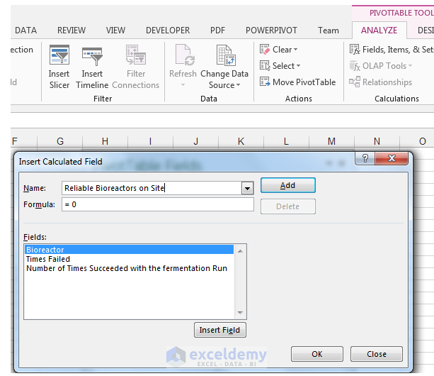
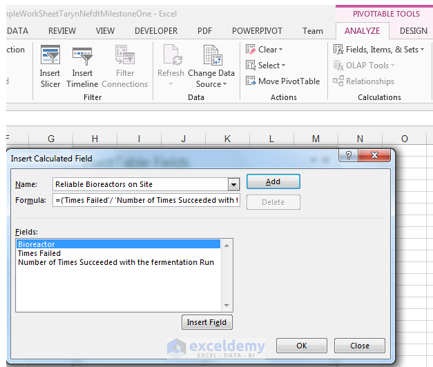
4) In the Formula field, instead of zero (make sure the equals is still there), open a parenthesis and then double-click the ‘Times Failed’ field from the Fields field to add it, and then divide this by the ‘Number of Times Succeeded with the fermentation run’, close parenthesis and then multiply by 100.
Then our formula will be:
= (‘Times Failed’/ ‘Number of Times Succeeded with the fermentation run’)*100
This formula will return our rate of failure.
5) And then click Add to see the new calculated field and then click OK.
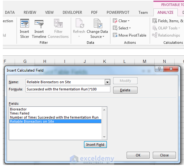
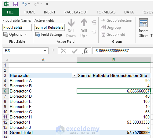
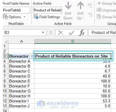
6) You should end up with something like the following:
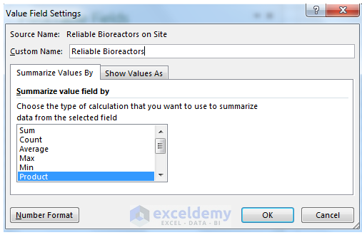
7) Go to Field Settings and from the Value Field Settings dialog box, choose Product, and click OK.
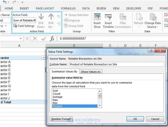
8) Go back to Field Settings and the Value Field Settings dialog box should be shown.
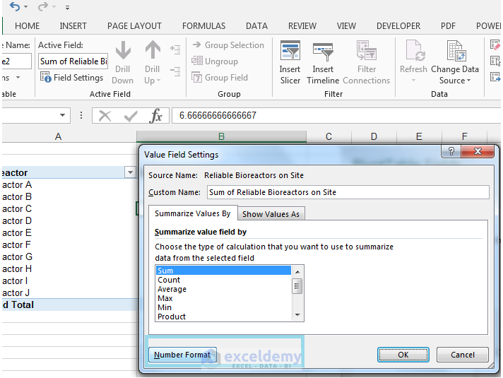
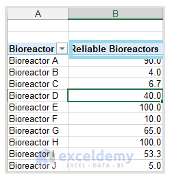
9) Click on the Number Format, select Number (already selected), and then set the decimal places to 1, and then you have it.
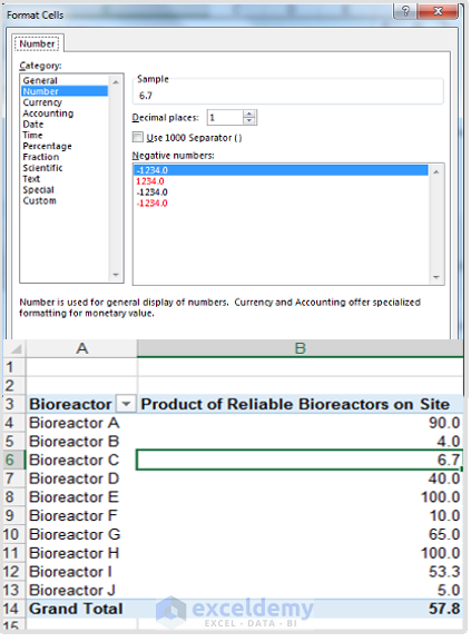
10) So, we can see from our data that Bioreactor A, H, and E had the highest failure rates and the company should not be ordering equipment from those suppliers in the future.
Pivot Table Calculated Field with IF Statement
Now, let’s see how to make a more complex calculated field.
Say our original data set has been updated to include a ‘Microorganism Used’ column in the source data, this is the microorganism in the bioreactor that is responsible for producing the biofuel and other products.
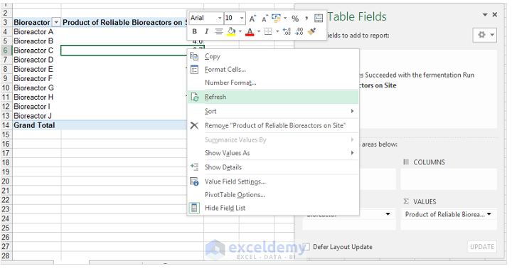
We can select a cell in the Pivot Table and right-click to Refresh, in order to see the updated fields from the source data.
We want a more complex calculated field that looks at the number of times the fermentation run succeeded, irrespective of the failure. If the fermentation run succeeded more than 50 times, it means the growth of the organism is fine and it’s reached optimum growth. If the number of times succeeded is less than 50, it means that the growth of the actual organism was problematic and the organism did not survive in the bioreactor.
Read More: How to Create an Average Calculated Field in Excel Pivot Table
We then follow the same steps to create a calculated field as above, but this time we do the following:
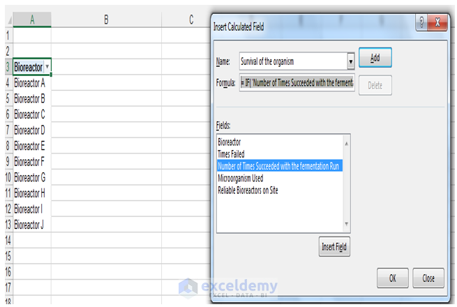
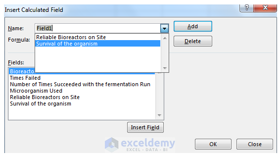
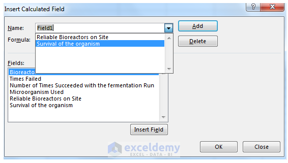
1) We give the Calculated Field the name ‘Survival of the organism’ as shown, and for the formula, we use an IF function based on the Number of Times Succeeded with the fermentation run Column
= IF( ‘Number of Times Succeeded with the fermentation Run’>=50,100%,0)
We click Add and then OK.
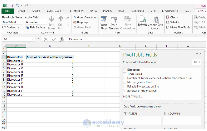
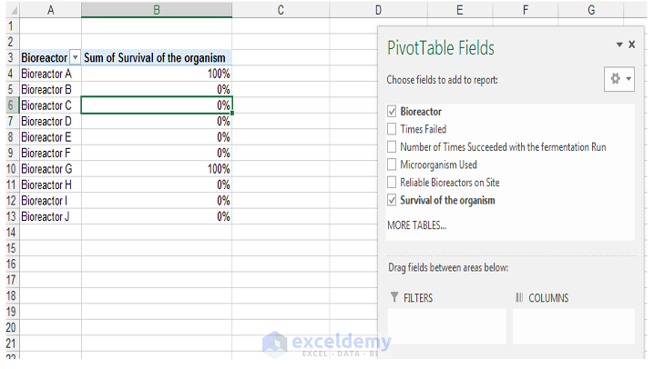
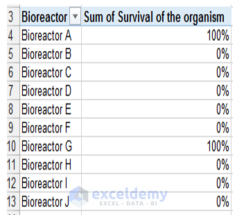
2) We now should have the following as shown below:
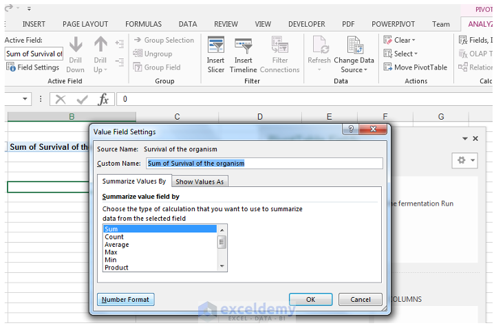
3) We then go to Field Settings in the Active Field Group.
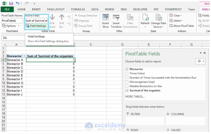
4) Choose Number Format from the Value Field Settings dialog box.
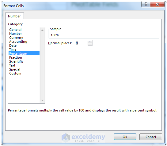
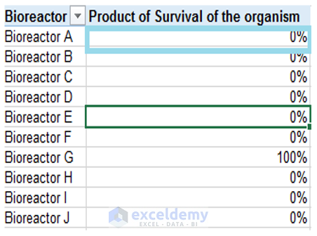
5) Click on Percentage and choose 0 decimal places, click OK and then OK again to close both dialog boxes, and then the values are in percentages instead of 1s and 0s.
6) There you have it, we can conclude that even though the bioreactor was failing in Bioreactor A’s case, the growth of the actual organism was fine.
Read More: Pivot Table Calculated Field for Average in Excel
Problems with Excel Pivot Table Calculated Field Tools
Totals are usually always a problem with Calculated Fields since Excel often does not Total them correctly. The best way to work around this is to hide the Totals column since it is just confusing and can make others looking at your Pivot Table, think you did something wrong. So, let’s hide the Totals Columns and Rows.
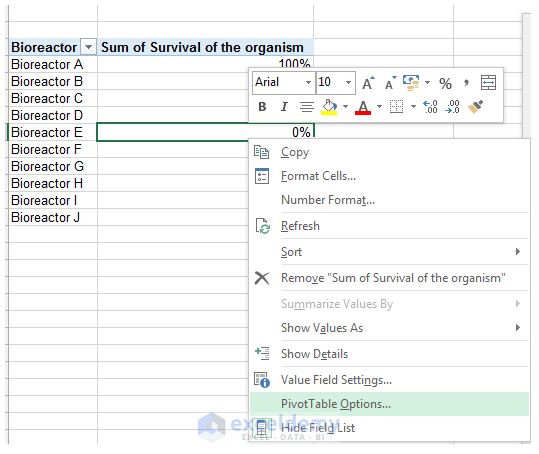
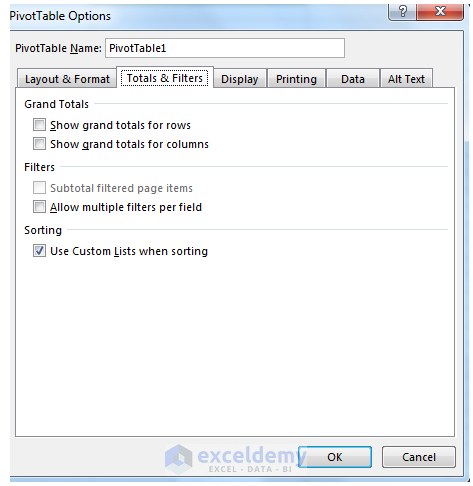
1) Right-click a cell in the Pivot Table and Choose PivotTable Options as shown.
2) In the PivotTable Options dialog box, in the Totals and Filters tab, Make sure Show grand totals for rows and Show grand totals for columns is unchecked.
3) The Incorrect Totals are then not shown.
Another common problem is the name of the field at times since Excel often adds the “sum” or “product” text as a part of the title.
1) In the ∑ Values of the PivotTable Fields dialog box, click on the drop-down arrow next to Product of Reliable Bioreactors on Site.
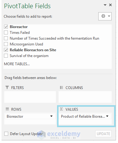
2) Go to Value Field Settings…………
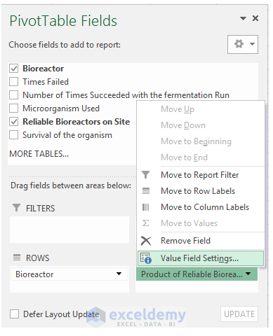
3) Change the Custom Name in the Value Field Settings and remove “Product” and type Reliable Bioreactors instead as shown.
4) Click OK.
How to Edit Calculated Field?
So, what happens when we want to modify or edit a calculated field that we already created for the Pivot Table, well we can easily do this.
Read More: Excel Pivot Table Terminology
1) Make sure you have a cell in the Pivot Table selected to activate the context-sensitive PivotTable Tools Analyze tab. In the Calculations Group, choose Fields, Items & Sets and select Calculated Field as shown.
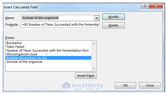
2) Click on the drop-down arrow next to Name and select one of the calculated fields you created previously.
3) In this case, we will select Survival of the organism calculated field we created recently.
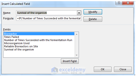
4) Then adjust the formula, in this case, we are going to enter this modified formula:
= IF(‘Number of Times Succeeded with the fermentation Run’ >=105,100%,0)
So, we are changing 50 to 105
5) Then click Modify and OK.
6) This is what the resultant Pivot Table looks like as a result of modifying the formula – we can see Bioreactor A is no longer included in the good growth rate, as a result of the change in the formula.
How to Delete a Calculated Field in a Pivot Table?
Deleting a calculated field in a Pivot Table is really easy.
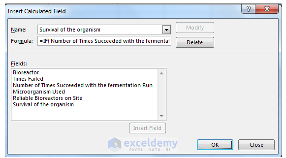
1) In the Analyze tab, of the PivotTable Tools, select Fields, Items & Sets drop-down and Calculated Field as shown.
2) Click the drop-down arrow next to Name and choose the name of the calculated field you created that you now want to delete. In this case Survival of the organism.
3) Click Delete as shown and OK.
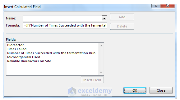
4) Then Survival of the organism is deleted completely in both the Calculated Field and Pivot Table Fields List.
Useful Pivot Table related Links from ExcelDemy
How to Use Pivot Table Data in Excel Formulas
How to Create Pivot Tables that Provide Meaningful Data Analysis & Insights [Dream Analysis]
8 Excel Pivot Table Examples – How to Make a PivotTable!
Conclusion
Calculated fields are extremely useful features when you need extra customization of the standard Pivot Table options. Calculated fields can be used for many unique calculations, which are not natively in Excel, but that may be required by your particular industry. Proceed with caution with TOTALS in the calculated fields options, since more often than not they need to be turned off, in order to not create confusion. Please feel free to comment and tell us what you have used calculated fields for and in which industry.
Useful links
Excel Pivot Table Tutorials for Dummies Step by Step
Download Working File
Calculated-Fields-Sample-WorkSheet.xlsx
Get FREE Advanced Excel Exercises with Solutions!
