How to Use Flash Fill in Excel (7 Easy Examples)

Flash Fill is one of the most important features in Excel. The beauty of Flash Fill is that separation happens within a flash and does not need any kind of formula. In this article, we will learn how to use Flash Fill in Excel with some simple examples. Let’s see the examples below.

Introduction to Excel Flash Fill

Flash Fill technique can recognize a pattern in a text and you can separate part of a text in a new column using this pattern recognition capability of Flash Fill. This feature is available in Excel 2013 and later versions.

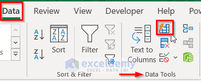
Location of Flash Fill in Excel

The Flash Fill tool is in the Data Tools group under the Data tab. The location is shown in the screenshot below.

Shortcut of Excel Flash Fill

The shortcut key for Flash Fill is: Ctrl + E

Flash Fill in Excel: 7 Easy Examples

This article will guide you with seven easy examples to use Flash Fill. To demonstrate the examples, we will use some simple datasets. Besides, we will describe the steps with screenshots so that you can easily understand them. So, without further delay, let’s get started.

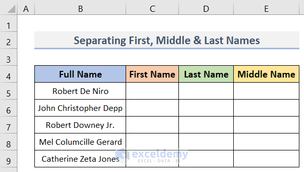
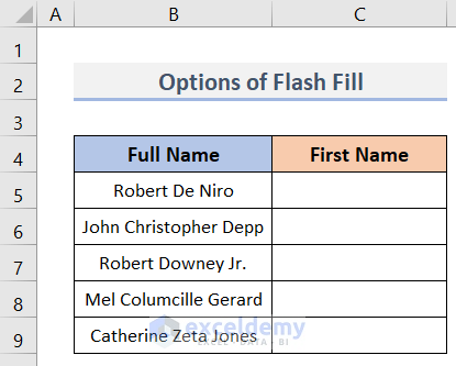
1. Separate First, Middle & Last Names

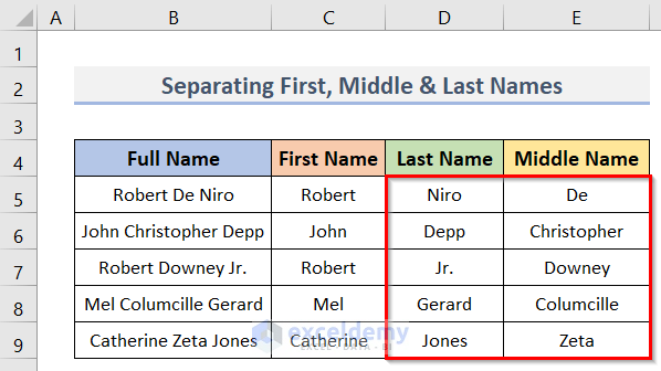
Let’s say, we have a dataset (B4:E9) in Excel that contains some Full Names in column B. For example, one name is ‘Robert De Niro’. Other names also consist of three parts like ‘Robert De Niro’. Now, we want to separate the First Name, Middle Name, and Last Name into separate columns. We can do it easily using Flash Fill. The steps are below.

Steps:

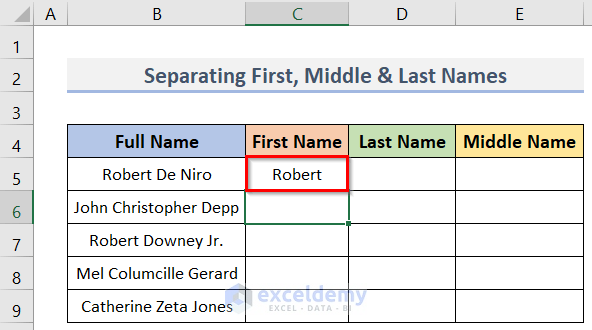
• To begin, enter the First Name in the column (cell C5 in column C) next to your data and press Enter.

• Next, start typing the next name (cell C6).
• Consequently, Flash Fill will suggest the first part of all names (C6:C9).

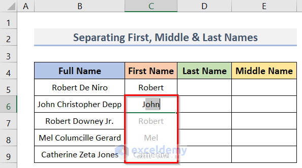
• If it is what you want, press Enter.
• Hence, we can see all the First Names in column C.

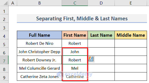
• Similarly, we can separate the Last Names and the Middle Names in columns D & E (see screenshot).

2. Split Text Using Flash Fill

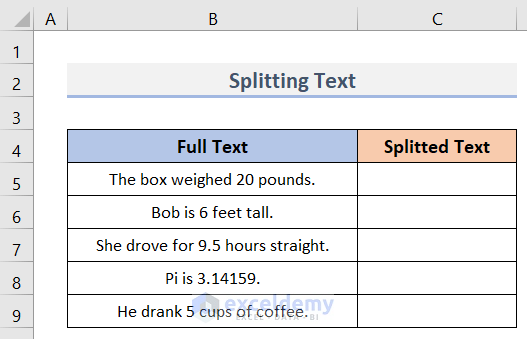
The Text to Columns wizard works very well for many types of data. But some data can’t be split by this wizard. For example, you can’t split data in this technique if it does not have a  fixed-width or the data doesn’t have delimiters. In this type of case, the Flash Fill feature can help you. For this, we will use the dataset (B4:C9) below containing some Texts (B5:B9) in a single column (B). Our goal is to extract the number part from each cell and put these numbers into a separate column (column C). The Text to Columns Wizard can’t do this separation because the space delimiters aren’t consistent here. It is because, in the first row, the number 20 is placed after 3 spaces, in the second row 6 is placed after 2 spaces, and so on. Therefore, we will use the Flash Fill technique to split the numbers properly. The steps are below.

Steps:

• First of all, click on cell C5 to select it.
• Then, enter the first number 20 in cell B1.

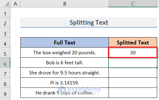
• After that, move to cell B2 and type the second number 6 in this cell.
• Now, go to the Data tab > Data Tools group > click on Flash Fill (or press Ctrl + E).

• Thereupon, you will see that the rest of the cells (C6:C9) are automatically filled by Excel.
• Finally, your new column will look like the following image.

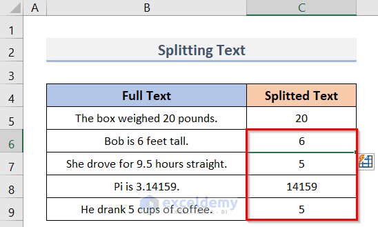
• As you see in the screenshot below, Excel has identified most of the numbers accurately.
• But some wrong guesses are also there.
• In cells C7 & C8, it just extracted the part after the decimal points.

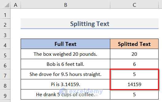
• To solve this issue, delete the suggested value (5) in cell C7.
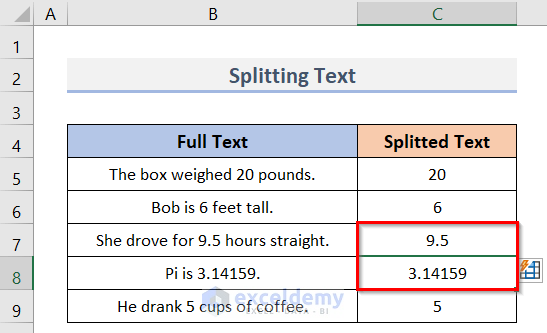
• Later, type the accurate value (9.5) in the cell (C7).

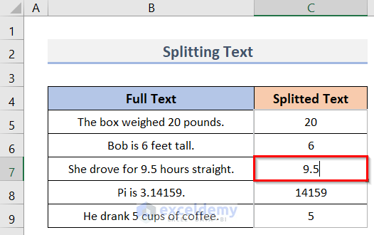
• Afterward, press Enter.
• Eventually, we will get the accurate number (3.14159) in cell C8 also.
• Thus, Excel identifies the pattern and suggests the correct numbers.
• See the following screenshot.

Read More: How to Use Flash Fill in Excel to Split Data

3. Apply Flash Fill to Merge Columns

Let’s say, we have a dataset (B4:E9) below that contains the names of some Fruits, Countries and the Order IDs of the fruits. Here, we will use the Flash Fill feature to merge the data in columns B, C, D and place it in column E. Moreover, Flash Fill can merge the values with space, comma, semicolon etc. Follow the steps below to do so.

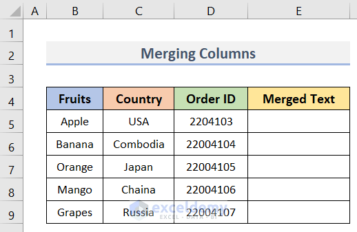
Steps:

• Firstly, go to cell E5.
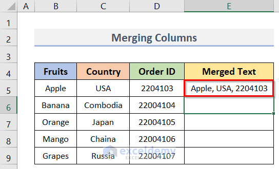
• Secondly, type the values in cells B5, C5 & D5 along with comma and space (see screenshot).
• Next, press Enter and you will automatically go to the next cell (E6).

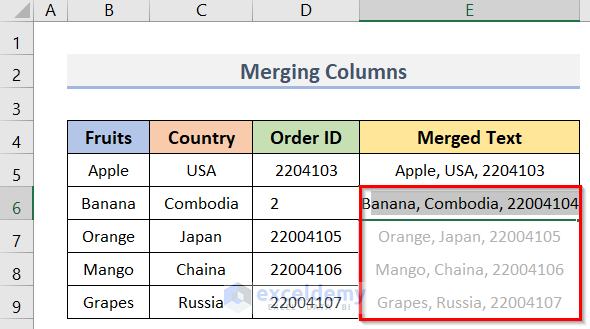
• Now, start typing the next Fruit (Banana) and you will see the suggestions in the range (E6:E9).
• The suggestions are of the same pattern as the merged data in cell E6.

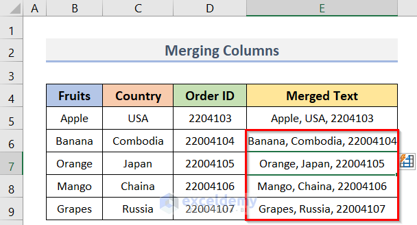
• Lastly, press the Enter button on the keyboard.
• In this way, you can merge all the data in the three columns (see screenshot).

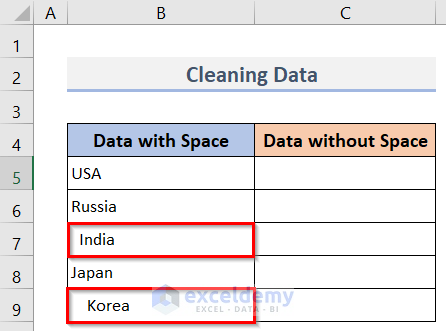
4. Clean Data with Flash Fill

Assuming, we have a dataset in Excel containing the names of some countries in the range B5:B9. Here, we can see that the data in cells B7 and B9 begin with some spaces. However, we can remove these spaces using the Flash Fill tool. The steps to do so are below.

Steps:

• In the first place, select cell C5.
• Then, type ‘USA’ without any space before it.

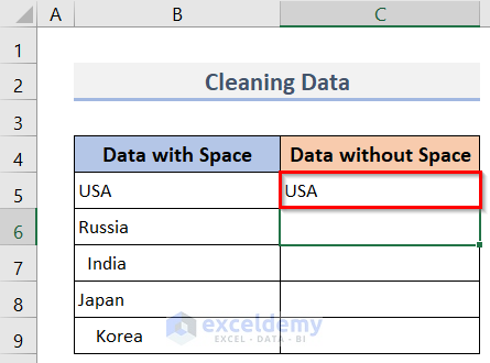
• Press the Enter key to move to the next cell (C6).
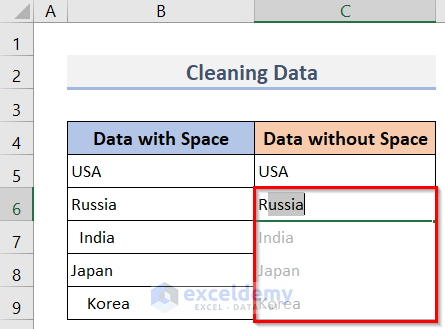
• Now, if you start typing the name of the next country (Russia), you will see the suggestions of all the countries below (C6:C9).

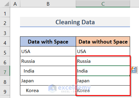
• If you press the Enter key, you will get all the countries without any space before them.
• Thus, we can clean the spaces before the data.
• See the following picture.

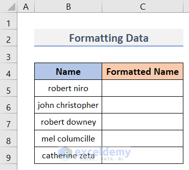
5. Excel Flash Fill to Format Data

In this example, we will apply the Flash Fill feature to format data in a worksheet. For describing this method, we will use the dataset below that contains some Names starting with lowercase. Here, we want to format these Names (both the first name & second name) so that they start in uppercase. Furthermore, we will insert commas and spaces between the first & second names. See the following steps.

Steps:

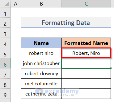
• In the beginning, select cell C5 by clicking on it.
• Next, type the Name of cell B5 in the same format shown in the image below.
• Press Enter.

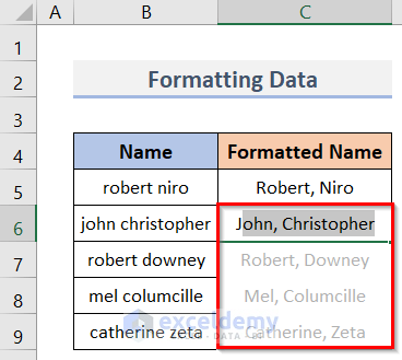
• Then, type the first letter (uppercase) of the next name (john christopher) in cell C6.
• Hence, all the names will be suggested in the same format (see screenshot)

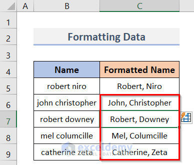
• After pressing the Enter button, you will get the rest of the names (C6:C9) in the same format specified in cell C5.

6. Create Email Addresses

Suppose, we have a dataset (B4:E9) in Excel. It contains some Names (B5:B9), IDs (C5:C9) and Domains (D5:D9). Here, we need to create email addresses using these given data. Again, we will use the Flash Fill tool to form the Email IDs in the range E5:E9. The steps are below.

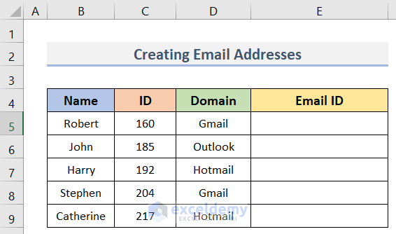
Steps:

• First, activate cell E5.
• Now, type the Email ID using the data in the B5:D5 range.
• A sample format of the Email ID is shown in cell E5 of the following screenshot.
• After that, press the Enter key.

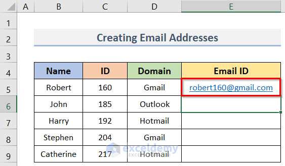
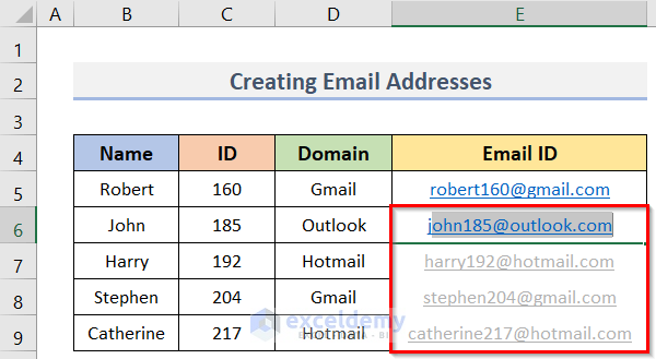
• Then, type the first letter (j) of the next name.
• Eventually, you will see the suggestion of the Email IDs for the cells (E6:E9) below.
• See the following image.

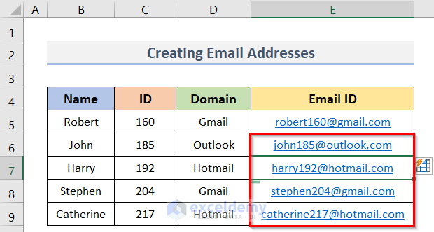
• Therefore, press the Enter key to accept the suggested Email IDs.
• In this way, you will get all the Email IDs at once.

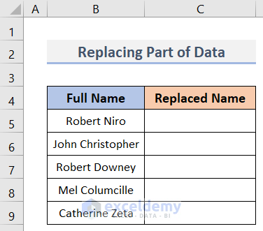
7. Replace a Part of Data Using Flash Fill

Let’s say, we have a dataset below containing some Full Names in the range B5:B9. Suppose, we want to replace the second names (for example, Niro) with ‘###’. We can do this easily with Excel’s Flash Fill technique. The steps to do so are below.

Steps:

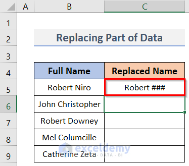
• First, select cell C5.
• Then, type ‘Robert ###’.
• Eventually, press the Enter key.

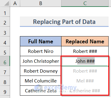
• Subsequently, type the first letter (J) of the second name in cell C6.
• As a result, you will see the suggestions of all the names in the same pattern specified in cell C5.

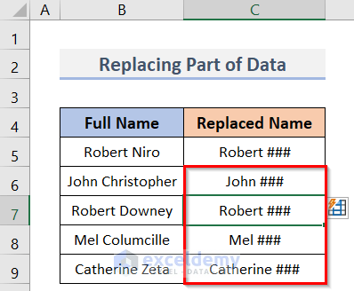
• Therefore, press the Enter key and accept the suggestions.
• Lastly, see the output in the screenshot below.

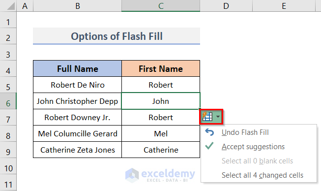
Flash Fill Options in Excel

To see the Flash Fill options, first of all, you will need a dataset. In our case, we will use the dataset (B4:C9) below. The steps to see the Flash Fill options are below.

Steps:

• In the beginning, apply any method of Flash Filling in the range C5:C9.
• Eventually, you will see the drop down menu of the Flash Fill beside column (C) where you applied Flash Fill.
• Now, click on the drop down menu.
• In this way, you can find the Flash Fill options.
• See the following image.

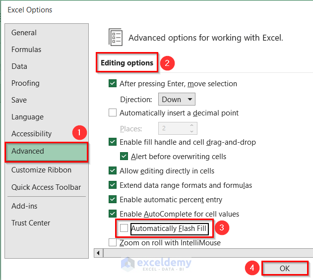
How to Turn Off Flash Fill in Excel

Sometimes, you may need to avoid the Flash Fill suggestions in Excel. You can do this by turning off the Flash Fill feature. Follow the steps below to do so.

Steps:

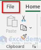
• Firstly, go to the File tab.

• Subsequently, click on the Options button.

• In turn, the Excel Options dialog box will appear.
• Eventually, click on Advanced > Editing options > uncheck the Automatically Flash Fill box > OK.
• See the steps in the following picture for a better understanding.
• In this way, we can turn off Flash Fill in Excel easily.

Limitations of Flash Fill in Excel

Though there are a lot of benefits of Flash Fill, there are some limitations too. They limitations are:

• The main limitation of using Flash Fill is, it is not a dynamic technique. If your data changes, columns created by Flash Fill do not update automatically (you must use a formula to update automatically then).
• Flash Fill ignores cells that contain non-printable data.
• Sometimes, it changes numbers into strings.

Things to Remember

While using the Flash Fill feature, you should always keep in mind the following points:

• You must check your data very carefully after using Flash Fill. If you get that the first few rows are correct, and assume that Flash Fill worked correctly for all rows, then a serious mistake may occur.
• Flash Fill works successfully only when the data is consistent.
• It increases accuracy when you provide more examples.

Download Practice Workbook

Download the practice workbook from here.

Conclusion

I hope the above tutorial will be helpful for you to use flash fill in Excel. Download the practice workbook and give it a try. Let us know your feedback in the comment section.

Flash Fill in Excel: Knowledge Hub

• Flash Fill Not Recognizing Pattern in Excel
• [Solved!] Flash Fill Not Working in Excel

<< Go Back to Learn Excel