In this post, you will learn how to calculate the running average of a data set. A business generates a considerable amount of data every year. Most of the data is related to time. One useful way to analyze your data is to find the average. For example, if you run a website or blog like me, you will count how many visitors are coming to your blog every month. This is an example; your business or website generates much more data. In this article, we shall learn how to calculate the Running Average in Excel.
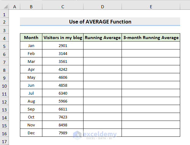
Let’s explain what the running average is with an example. In the image below, you will see an Excel workbook titled Running Average. In the Visitors worksheet, you are seeing some data. Under the Month column, there are twelve months: from Jan to Dec. Under the “Visitors in my blog” column, you see the total number of visitors coming to my blog every month. The blog visitors have increased almost three times in the month of November. In Jan it was around 3 thousand and in the month of November, it was around 8 thousand and 500 hundred.
1. Calculating Regular Running Average with Excel AVERAGE Function
There are many default Excel Functions that we can use to create formulas. The AVERAGE function helps us to find the average of specific cells with numbers. Therefore, follow the steps below to perform the task.
STEPS:
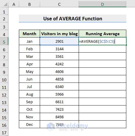
- First, select cell D5 and insert the AVERAGE function.
=AVERAGE($C$5:C5)- Here, I click cell C5 as the argument of the AVERAGE function.
- I’ll make the C5 reference an absolute reference, so press the F4 key on your keyboard.
- Thus, cell reference C5 turns into an absolute cell reference.
- Then, insert the range operator and again insert the C5 cell reference.
- Lastly, place the closing parenthesis after the formula.
- I press Enter.
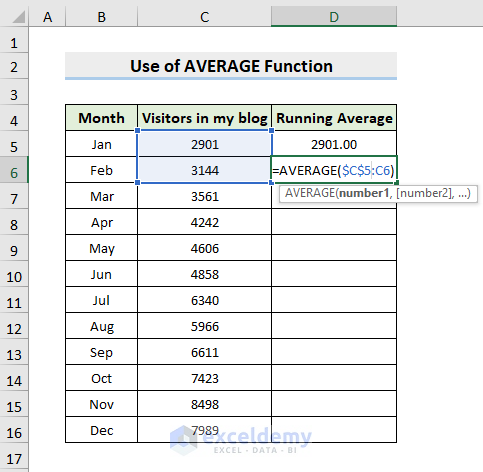
- The formula returns a value of 2901. This formula actually finds out the average of cell C5.
- Next, I select the cell and then copy the formula for the next cell.
- The formula returns 3022.5. I select the cell and click on the formula bar. You see this formula selects cells C5 to C6. So the formula calculates the average of cells C5 to C6. I am sure you are getting the idea of how the running average actually works.
- Now I copy the formula for other cells in the column.
- Afterward, I select the last cell and click on the formula bar. You see this formula works on all the cells in the column, from cells D5 to D16.
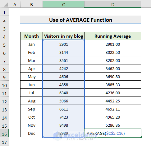
- So, this is how you can calculate the running average of some values.
Read More: Moving Average Formula in Excel
2. Calculating 3 Months Running Average in Excel
Moreover, we’ll show the process to get the ruining average of 3 months which is more practical for any business. So, learn the following steps.
STEPS:
- Under the 3-month Running Average column, I select the third cell E7. As we are going to find out the running average of 3 months, we have to start from the third month. You cannot find out 3-month running averages using only 1 or 2 values. The formula is:
=AVERAGE(C5:C7)- Here, I insert the average function in cell E7, I select cells C5 to C7. This time I am not going to turn any cell references to absolute as when I copy this formula to the cells below, I want every formula will select the last three values.
- So I close the function and press Enter.
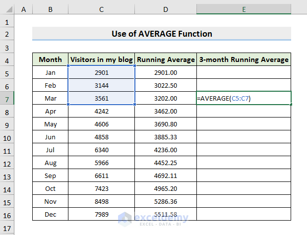
- Consequently, the formula returns 3202. It is the same as this running average. The reason is this running average finds out the average of these three values and this 3-month running average also does the same.
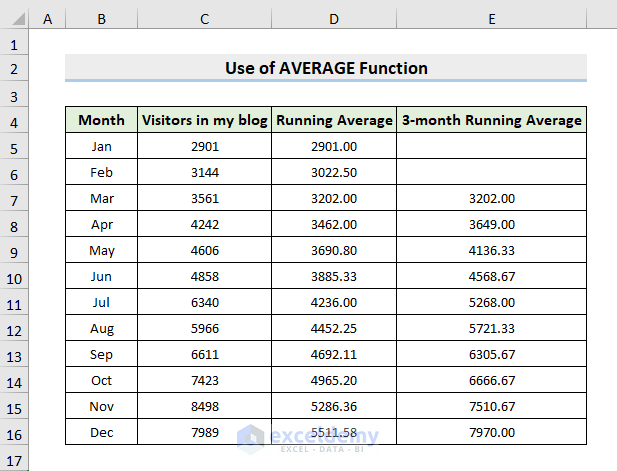
- Now I copy the formula to other cells in the column.
- In this way, you’ll get all the 3-month running averages.
3. Inserting Excel SUM Function to Determine Running Average
However, you can use the SUM function and the COUNT function in Excel to determine the average of some values. Hence, follow the process.
STEPS:
- Firstly, select cell D5.
- Then, insert the formula:
=SUM($C$5:C5)/COUNT($C$5:C5)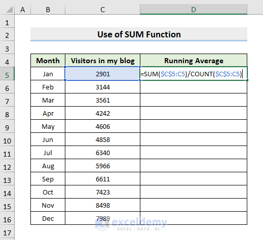
- Subsequently, press Enter.
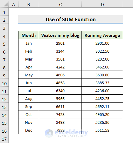
- After that, use AutoFill to fill in the rest.
- Hence, it’ll return the running averages in cells D5 to D16.
Read More: Calculate Moving Average for Dynamic Range in Excel
Download Practice Workbook
Download the following workbook to practice by yourself.
Conclusion
Henceforth, you will be able to calculate the running average in Excel following the above-described examples. Keep using them and let us know if you have more ways to do the task. Don’t forget to drop comments, suggestions, or queries if you have any in the comment section below.
Related Articles
- Excel Formula to Find Displaced Moving Average
- How to Calculate Exponential Moving Average in Excel
- How to Calculate 7 Day Moving Average in Excel
- How to Calculate Centered Moving Average in Excel
- How to Generate Moving Average in Excel Chart
- How to Determine Triple Exponential Moving Average in Excel
<< Go Back to Moving Average | Calculate Average in Excel | How to Calculate in Excel | Learn Excel
Get FREE Advanced Excel Exercises with Solutions!

I love this article very much and I am just learning it for the first time.
Thanks.
Great explanation. I used it and it worked. Thanks for the insights.