Excel Pivot Table Formatting (The Complete Guide)

PivotTable helps you summarize your data quickly and easily. With the help of Excel pivot table formatting, you can display the analyzed data perfectly.

In this article, you will learn about Excel pivot table formatting. There are different ways of doing that.

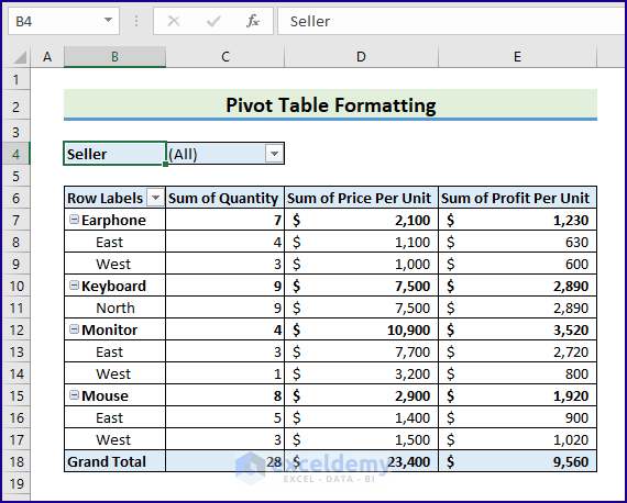
Selecting a PivotTable cell displays two additional tabs; PivotTable Analyze and Design, along with other Excel tabs. Using those tabs, you can apply or modify Excel pivot table formatting to make your data more presentable.

Follow the below sections to learn about different aspects of pivot table formatting.

1. Formatting Number in Pivot Tables

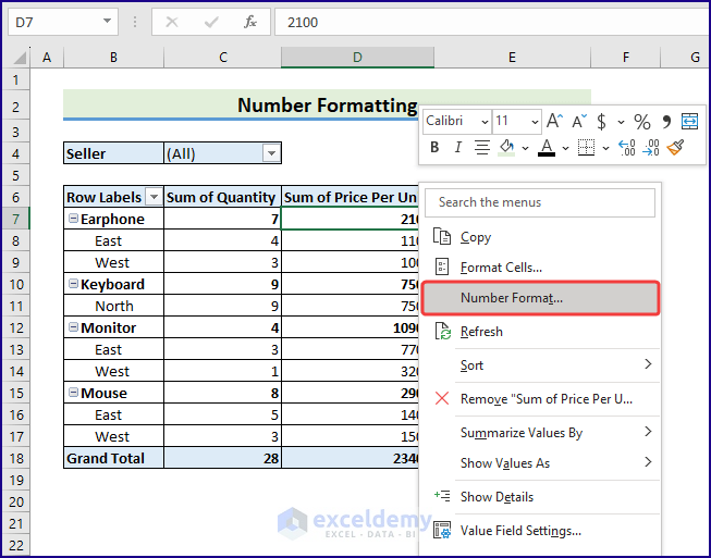
The pivot table uses General number formatting. You can change the number format for all the pivot data.

To change the data format, right-click any value >> choose Number Format from the shortcut menu.

Then use the Format Cells dialog box to change the number format of your pivot data.

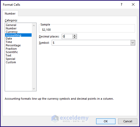
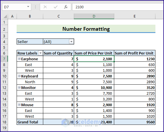
Then, all the cells of the group will be formatted as accounting.

2. Pivot Table Designs

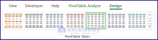
There are several built-in styles that you can apply to your pivot table.

Select any cell in your pivot table and then choose Design > PivotTable Styles to select a style.

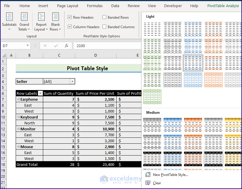
2.1 More Pivot Table Designs

If these styles don’t fulfill your purpose, you can choose more styles by clicking on the following button.

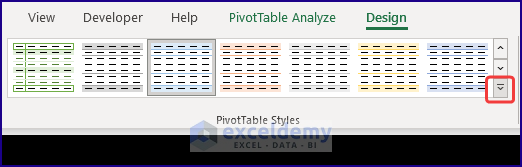
You will find lots of built-in styles for you to use in your pivot tables.

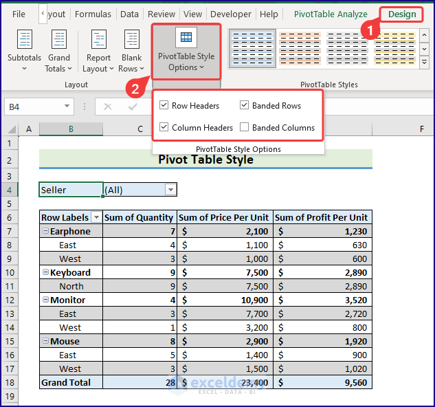
2.2 Tuning Pivot Table Styles

You can fine-tune your styles using controls in the Design > PivotTable Style Options group.

2.3 Layout Controls in Excel Pivot Tables

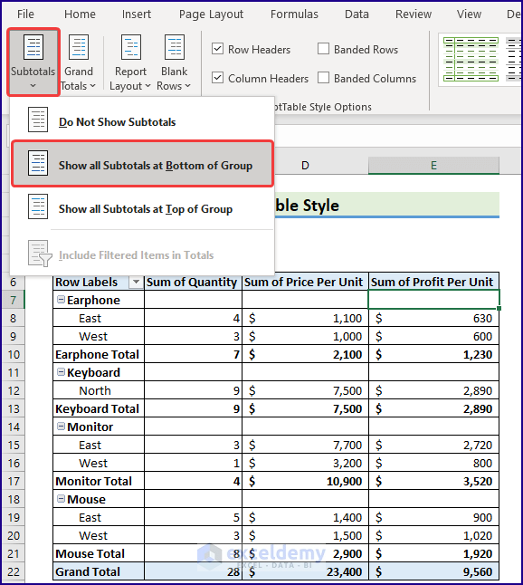
You can also use the controls from the Design > Layout group to control various elements in your pivot table. You can use any of the following controls:

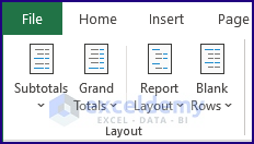
Subtotals: Using this control, you can add/ hide subtotals and choose where to display them (above or below the data).

Grand Totals: Using this control, you can choose which types, if any, to display.
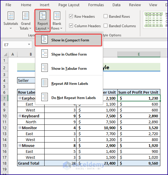
Report Layout: There are three report layouts. You can choose any of the three different layout styles (compact, outline, or tabular) using this control. You can also choose to hide/active repeating labels.

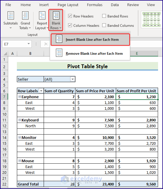
Blank Row: You can add a blank row between items to improve readability.

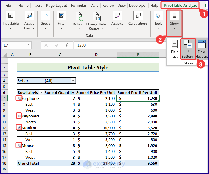
3. Field Controls of Pivot Tables

The PivotTable Analyze > Show group contains more options that affect the appearance of your pivot table. For example, you use the Show +/- Button to toggle the display of +/- sign in expandable items.

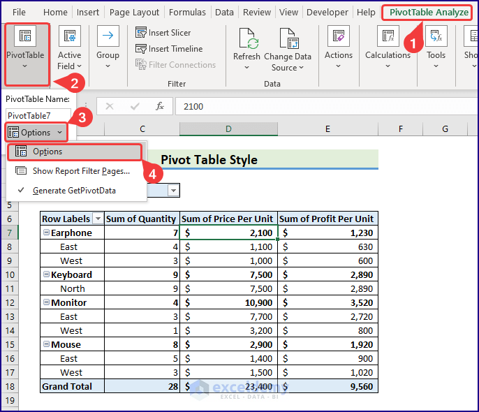
4. PivotTable Options Dialog Box

Still, more pivot table options are available from the PivotTable Options dialog box.

To display this dialog box, choose PivotTable Analyze > Options (in the PivotTable section) > Options.
Or you can right-click any cell in the pivot table and choose PivotTable Options from the shortcut menu.

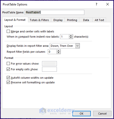
The PivotTable Options dialog box will be visible now.

Experimenting with styling features is the best way to become familiar with all these layout and formatting options.

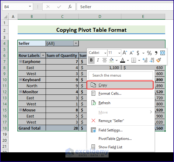
5. Copying a Pivot Table Format

If you want to copy the format of your pivot table in other worksheets or in your existing worksheet. You can do the following.

Select the Pivot Table >> right-click on the mouse >> select copy from the menu.

Select a range in your existing worksheet or new worksheet where you want to paste your data. You can paste the data directly into the available paste option or you can use the paste special feature.

Select any cell >> Right-click on the mouse >> Choose Paste Special.

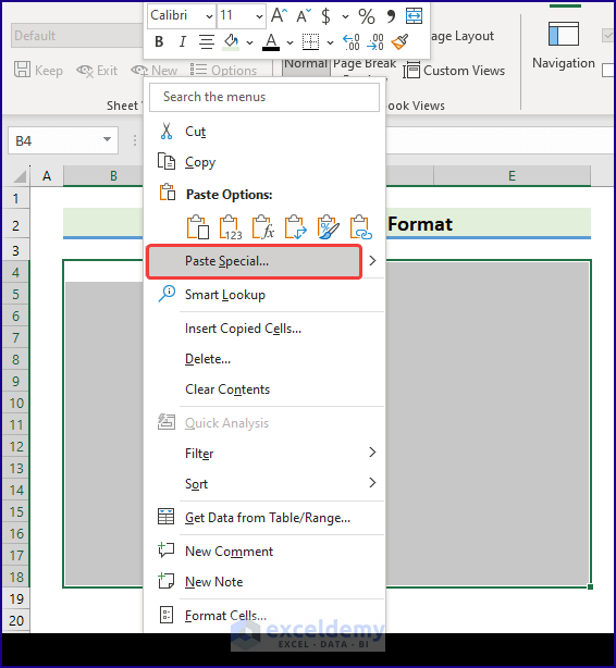
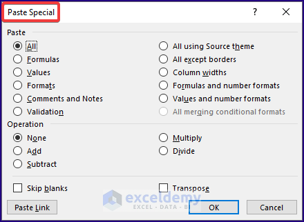
In the Paste Special feature, click on the paste option that you want to use and click OK.
Here, I selected All from Paste.

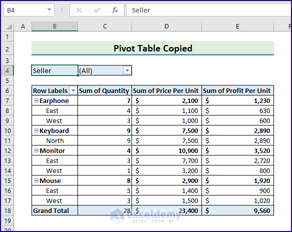
So, Excel has copied the Pivot table data with all formatting.

6. Locking Pivot Table Format

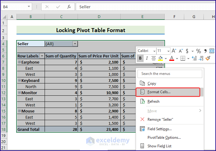
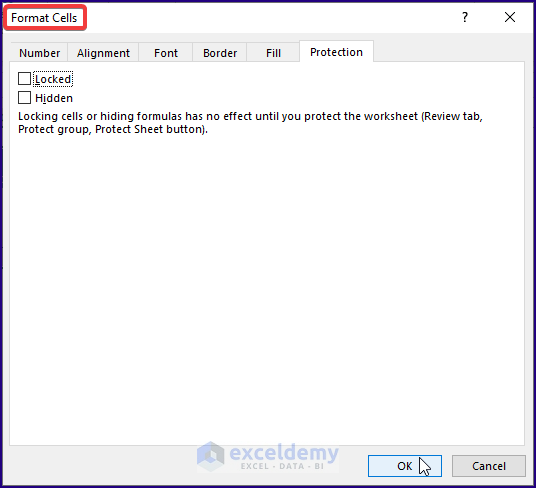
First, select the entire pivot table and right-click your mouse >> click the Format Cells option.

In the protection option of the Format Cells Uncheck the Locked option and press OK.

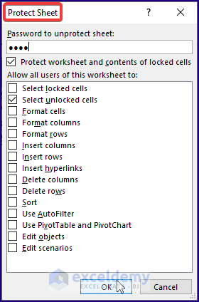
Then on the Review Tab on top, click on the Protect Sheet
Put a tick mark on the Select unlocked cells and set a password.

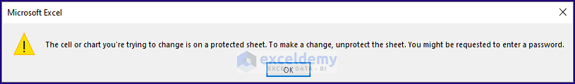
After this, whenever you want to edit the pivot table, a dialogue box will appear like in the picture below.

If you want to unlock the protected cells, click on the Review on top and then click on the Unprotect Sheet.
It will ask for a password (if you set one). Type the password. You will see the sheet is unlocked now.

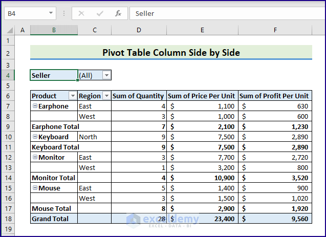
Pivot Table Column Side by Side in Excel

When you create a Pivot table, Excel will organize the row labels in one column only. But if you need to keep the row labels on the same line in Pivot Table and put the column side by side, you can rearrange them.

Select a cell in Pivot Table >> go to the Design tab >> click the dropdown of Report Layout >> select Show in Tabular Form.

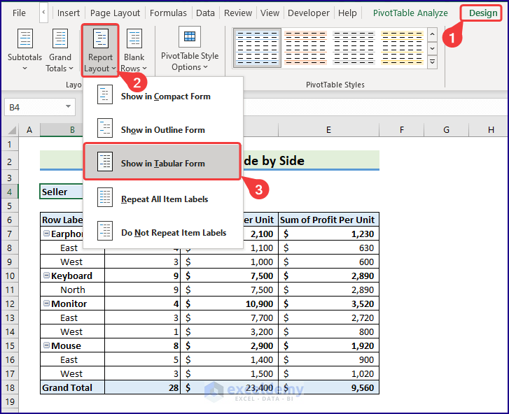
Your Pivot Table will rearrange itself by putting the columns side by side.

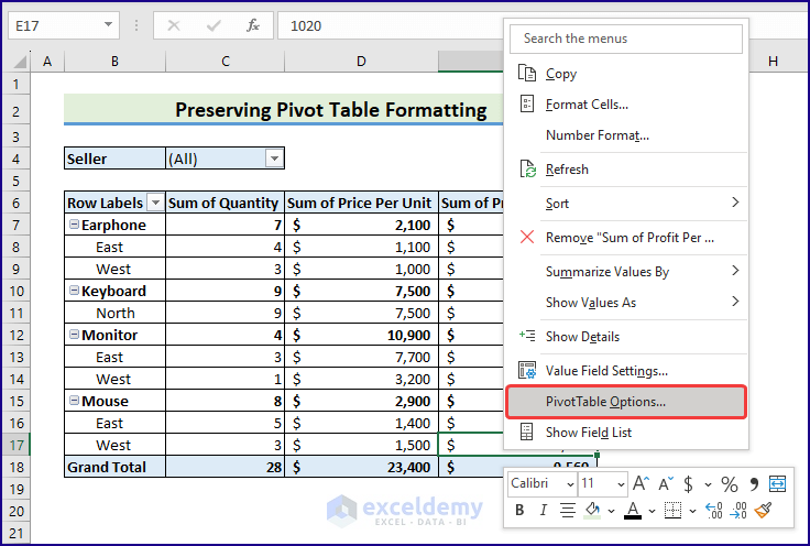
Pivot Table Formatting Not Preserved in Excel

Sometimes an unwanted situation like cell formatting in Pivot Table is not preserved and keeps changing and this may bother you. Well, accidentally you may have changed a configuration which you need to fix now.

Right-click on a cell in the Pivot Table >> select Pivot Table Options from the menu list.

The Pivot Table Options dialog box will appear.
Put a checkmark on Preserve cell formatting on update field if not checked.
Click OK.

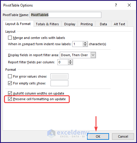
Your problem is fixed! As simple as that.

Frequently Asked Questions

1. Is it possible to change the date format in Pivot Table?

Obviously. Several ways are available to change the date format in Pivot Table.

2. How many types of layouts are in a Pivot Table?

In general, pivot tables typically have 3 types of layouts: tabular layout, compact layout, and outline layout.

Takeaways from the Article

To make your pivot tables more effective, it’s important to maintain a consistent style throughout the table. This includes using the same font, font size, and color scheme.
Use formatting options such as bold text or shading to draw attention to important data points in your pivot table.
It’s important to keep your pivot table clean and easy to read. Avoid overcrowding the table with too many columns or rows.

Download Practice Workbook

You can download the practice book from the link below.

Pivot Table Formatting.xlsx

Conclusion

This article demonstrates options to apply or change Excel pivot table formatting. Different aspects of pivot table formatting and their applicability are discussed. We hope this article sheds enough light on pivot table formatting to fulfill your requirements. Comment if you need further explanation or anything to add. Have a nice day!

Pivot Table Formatting : Knowledge Hub

<< Go Back to Pivot Table in Excel | Learn Excel

Get FREE Advanced Excel Exercises with Solutions!