While working with Excel, users have to deal with various Excel functions for their working purposes. These functions are mainly used for analysis or to reach a conclusion about their respective data. One such most-used function of Excel is the VLOOKUP function. In this article, I will show you various examples of the VLOOKUP function in Excel.
Examples of VLOOKUP Function in Excel: 7 Ideal Examples
In this article, you will see seven ideal examples of the VLOOKUP function in Excel. Users use the VLOOKUP function mainly for searching data from a data range with certain criteria. I will include not only the basic uses but also some advanced formulas to find values that require the help of the VLOOKUP function.
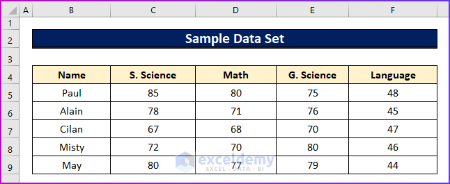
I will use the following sample data set to describe the aforementioned examples.
Read More: 10 Best Practices with VLOOKUP in Excel
Example 1: Search for Particular Value
The first example will demonstrate to you the most basic use of the VLOOKUP function. Here, I will find the marks of a certain person. See the following steps for a better understanding.
Steps:
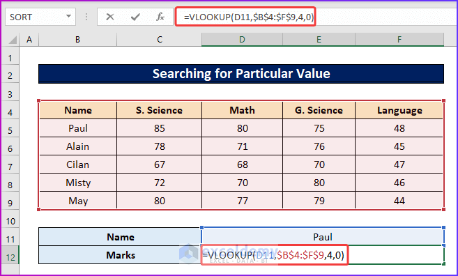
- First of all, look at the following image, where I want to find out the marks of Paul in his G. Science exam.

- Next, to do that, insert the following formula in cell D12.
=VLOOKUP(D11,$B$4:$F$9,4,0)- Here, the formula will search the name of cell D11 in the cell range of B4:F9, and then after finding the match, it will show the value from the fourth column of the data range that contains the marks of the G. Science of all the students.
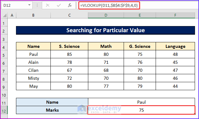
- Then, after pressing Enter, it will show the marks of Paul from that particular column.
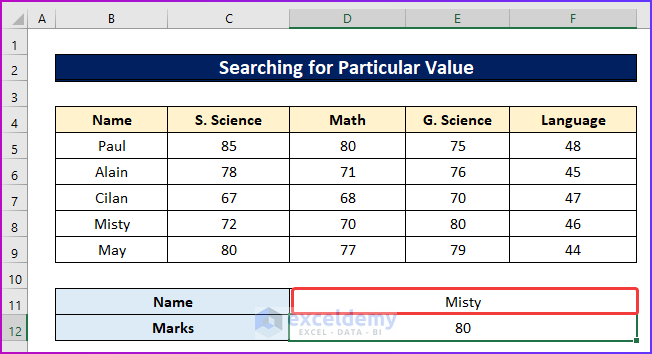
- Consequently, if you input any name in cell D11 from the value of cell range B5:B9 it will show the marks of that respective person.
Example 2: Perform Dynamic Search
In the previous example, the formula of the VLOOKUP function will only show values for the name and only one subject. What will be the procedure when you want to find out the marks for more than one lookup criteria? The following two segments address this issue by modifying the formula of the VLOOKUP function. Performing a two-way or three-way lookup is considered one of the best examples of the VLOOKUP function in Excel.
Read More: How to Make VLOOKUP Case Sensitive in Excel
Example 2.1: Execute Two-Way Lookup
In the first segment, you will see the process of doing a two-way lookup. Here, I will find out the marks of a certain subject of a specific person by using the VLOOKUP function formula. See the following steps.
Steps:
- First, like the following GIF, make three extra fields for the name of the person, the subject, and the marks.
- Next, in cell D13 use the following formula.
=VLOOKUP(D11,$B$5:$F$9,MATCH(D12,$B$4:$F$4,0),0)- Then, after pressing Enter, it will show the marks for the G. Science exam in May.
- Finally, if you change any value in cell D11 or D12 the value of cell D13 will change accordingly.
Formula Breakdown
=VLOOKUP(D11,$B$5:$F$9,MATCH(D12,$B$4:$F$4,0),0)
- First, the MATCH function will look for the cell value in column range B4:F4 and will return its relative position.
- Then, the VLOOKUP function will look in that particular column for the score of the specific person in cell D11.
Read More: How to Apply Double VLOOKUP in Excel
Example 2.2: Employ Three-Way Lookup
After doing the two-way lookup, you will see the example of a three-way lookup in this segment. Here, instead of considering two criteria, I will take three lookup criteria for this example. Let’s do this by following the below-given steps.
Steps:
- In the beginning, take a sample like the following data set where I have the marks of two-term exams of some students.
- Here, I want to find out the marks of each student based on three different criteria.
- To do that, in cell D23 write the following formula.
=VLOOKUP(D21,CHOOSE(IF(D20="First Term Exam",1,IF(D20="Final Exam",2,3)),B6:F10,B14:F18),MATCH(D22,B5:F5,0),0)- Then, you will see the value of the marks after pressing Enter.
- Finally, the result of the formula will change if you change any value of cells D20, D21, or D22 like in the following image.
Formula Breakdown
=VLOOKUP(D21,CHOOSE(IF(D20=”First Term Exam”,1,IF(D20=”Final Exam”,2,3)),B6:F10,B14:F18),MATCH(D22,B5:F5,0),0)
- First, the MATCH function will look for the subject name.
- Next, the IF function checks the type of exam from cell D20 and will return the range of marks depending on that exam and the subject name, and then the CHOOSE function selects the right range of values.
- Then, the VLOOKUP function will match the cell value of D21 and return the marks of the respective subjects of that respective term exam.
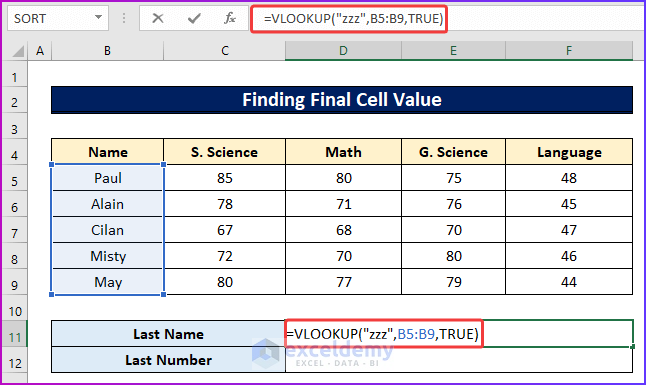
Example 3: Find Final Cell Value
Another example of the VLOOKUP function in Excel is to find the final cell value of a specific column. This value can either be a number or a text. I will show the process of finding both types of values in the following steps.
Steps:
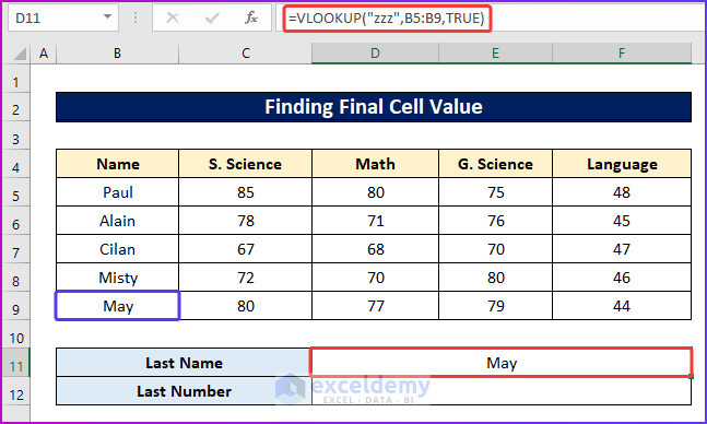
- First of all, to find out the last cell value that is a text, type the following formula in cell D11.
=VLOOKUP("zzz",B5:B9,TRUE)- Here, the “zzz” string in the formula is acknowledged as the largest of any names or texts that you can write with alphabets, so inserting this in the formula will always show the last text from a given cell range.
- Secondly, after pressing Enter you will get your desired name.
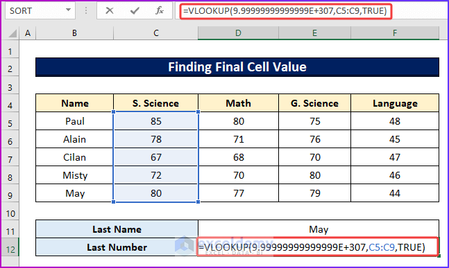
- Consequently, to get the last cell value of a range that contains a number use the following formula in cell D12.
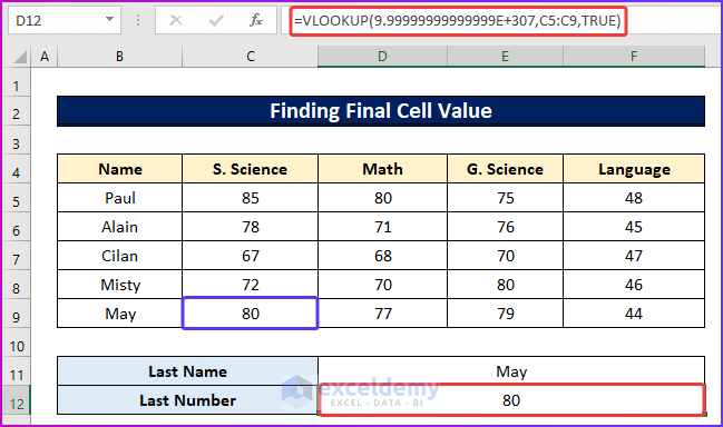
=VLOOKUP(9.99999999999999E+307,C5:C9,TRUE)- Here, from the formula, the term or the value “9.99999999999999E+307” is considered the biggest numerical value in Excel. So, after using this term in the formula will get the last value of a cell range that is a number.
- Finally, hit Enter and get the result of the above formula.
Related Content: How to Use Dynamic VLOOKUP in Excel
Example 4: Cary Out Partial Lookup
By using the VLOOKUP function, you can also do a partial lookup. For that, you need to insert wildcard characters of Excel like an asterisk (*) in your formula. The following steps with this example.
Steps:
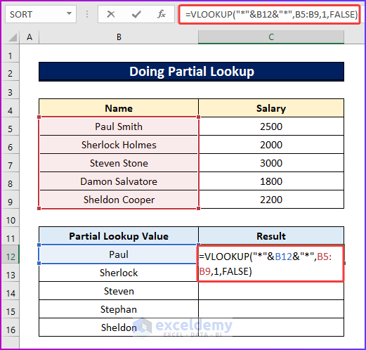
- In the beginning, look at the following image where the primary data set contains the full name but the secondary does not.
- In order to get the exact match of the names in the secondary data set with the primary ones, in cell C12, use the following formula.
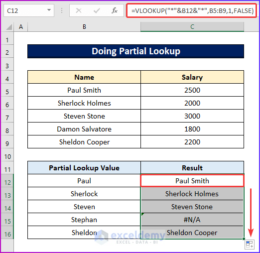
=VLOOKUP("*"&B12&"*",B5:B9,1,FALSE)- Here, in the formula by using the asterisk sign before and after B12, the formula will look only for the exact match of the cell value B12 in the cell range B5:B9 and show the result based on that match.
- Secondly, use Enter and then drag the formula using AutoFill to get all the desired results.
- Here, any name that does not match the values of the given cell range will get #N/A as a result.
Example 5: Handle Errors with VLOOKUP Function
If you don’t want to show #N/A as a result, when the VLOOKUP function doesn’t get an exact match then this example will be helpful for you. Follow the simple steps below to mitigate your issue.
Steps:
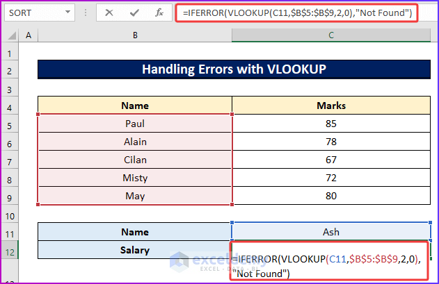
- Firstly, suppose you have a name in cell D11 that doesn’t match the values of your lookup range.
- In order to show the result of the name as not found, in cell D12, use the following formula.
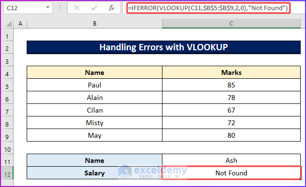
=IFERROR(VLOOKUP(C11,$B$5:$B$9,2,0),"Not Found")- Here, the IFERROR function will check if the result of the VLOOKUP function is true or not.
- If it finds the result false then will show Not Found as a result.
- Secondly, press Enter to get the result which is negative for this case.
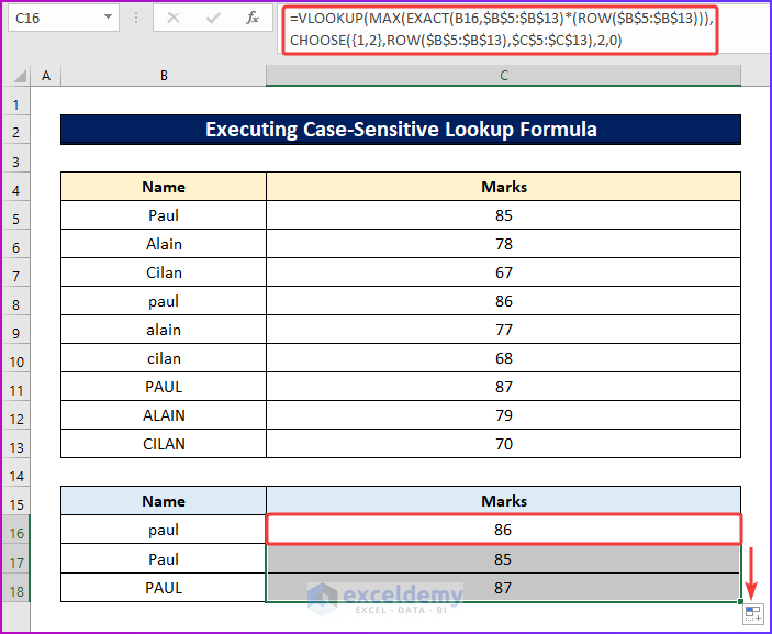
Example 6: Execute Case-Sensitive Lookup Formula
One major issue with the VLOOKUP function is that it is not case-sensitive. When you have the same names in different cases, the function will always get the first name, despite the given syntax. Solving these kinds of problems is one of the examples of the VLOOKUP function in Excel. To get through the issue, see the following steps.
Steps:
- Firstly, as you go through the following image, you can see the data set with three types of names.
- All of these names are the same but in different cases and their respective marks are also different.
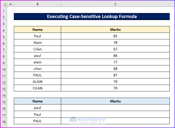
- In order to find the marks for the individual by considering the cases in their names, you have to insert the following formula for the first name in cell C16.
=VLOOKUP(MAX(EXACT(B16,$B$5:$B$13)*(ROW($B$5:$B$13))),CHOOSE({1,2},ROW($B$5:$B$13),$C$5:$C$13),2,0)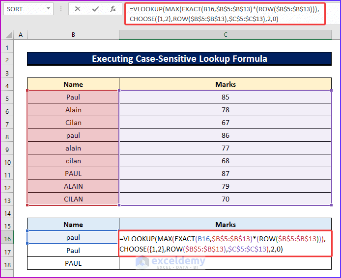
Formula Breakdown
=VLOOKUP(MAX(EXACT(B16,$B$5:$B$13)*(ROW($B$5:$B$13))),CHOOSE({1,2},ROW($B$5:$B$13),$C$5:$C$13),2,0)
- First, the EXACT function will look for an exact match of the cell value of B16 in the cell range B5:B13.
- Next, the result from the previous step will be multiplied by the ROW function and return the row number for the exact match of the previous step in an array.
- Then, the VLOOKUP function will match the cell value of D21 and return the marks of the respective subjects of that respective term exam.
- Then, after pressing Enter the above formula will show the result for that particular name.
- Consequently, use the Fill Handle to drag the formula to the lower cells to get the results of the following names.
Example 7: Perform VLOOKUP with Multiple Criteria
The last example of this article describes the VLOOKUP function formula for multiple criteria. The following steps of this discussion will help you perform this task easily.
Steps:
- Suppose, you have a data set like the following GIF where you have some students’ names and their marks in two-term exams.
- From here, I will find the marks of each student in those two exams.
- In order to do that, type the following formula in cell C17.
=VLOOKUP($B17&"|"&C$16,CHOOSE({1,2},$B$5:$B$14&"|"&$C$5:$C$14,$D$5:$D$14),2,0)- Then, after pressing Enter, you will see the first term marks of Paul in C17.
- Finally, drag the formula to the bottom and then to the right to see all the marks of all the students.
Formula Breakdown
=VLOOKUP($B17&”|”&C$16,CHOOSE({1,2},$B$5:$B$14&”|”&$C$5:$C$14,$D$5:$D$14),2,0)
- First, the CHOOSE function will give the values from each column from B:D of the cell range B5:D14 one by one.
- Next, the VLOOKUP function will match the cell values of B17 and C16 with the data from the previous result and will find an exact match to show the final result.
Things to Remember
- Remember to give the correct lookup range and col index number reference in the formula. Otherwise, you will not get your desired result.
- While searching with the VLOOKUP function formula, be careful about the exact match and case sensitivity, as the function is not case sensitive and will always show the first value that matches the criteria despite not matching the case.
- If you are not using Microsoft Office 365 then you have to press Ctrl + Shift + Enter instead of only Enter to get the result from an array formula.
Download Practice Workbook
You can download the free Excel workbook here and practice on your own.
Conclusion
That’s the end of this article. I hope you find this article helpful. After reading the above description, you will be able to understand the examples of the VLOOKUP function in Excel. Please share any further queries or recommendations with us in the comments section below.
We are always concerned about your preferences. Therefore, after commenting, please give us some moments to solve your issues, and we will reply to your queries with the best possible solutions.
Related Articles
- VLOOKUP Example Between Two Sheets in Excel
- Transfer Data from One Excel Worksheet to Another Automatically with VLOOKUP
- VLOOKUP from Another Sheet in Excel
- How to Use VLOOKUP Formula in Excel with Multiple Sheets
- How to Remove Vlookup Formula in Excel
- How to Apply VLOOKUP to Return Blank Instead of 0 or NA
- How to Hide VLOOKUP Source Data in Excel
- How to Copy VLOOKUP Formula in Excel
<< Go Back to Excel VLOOKUP Function | Excel Functions | Learn Excel
Get FREE Advanced Excel Exercises with Solutions!
