This is the If you are looking for special tricks to know about the OFFSET function with examples in Excel, you’ve come to the right place. This article will discuss the details of all the examples of the OFFSET function. Let’s follow the complete guide to learn all of this.
Download Practice Workbook
Download this practice workbook to exercise while you are reading this article. It contains all the datasets in different spreadsheets for a clear understanding. Try it yourself while you go through the step-by-step process.
Overview of OFFSET Function
The OFFSET function returns a reference to a range that is a given number of rows & columns from a given reference. The function starts with a cell reference, moves to a specific number of rows down, then to a specific number of columns right, and extracts a section out of the data set.
In this way, it returns a section of data with a specific height and width, situated at a specific number of rows down and a specific number of columns right from a given cell reference.
The function will move the specified number of rows upward from the reference cell if the rows argument is negative.
The Syntax of the OFFSET function is:
=OFFSET(reference,rows,cols,[height],[width])
Here, reference indicates the cell reference from where it starts off moving.
Rows dictate the number of rows it moves downward.
Cols illustrate the number of columns it moves rightward.
Height indicates the number of rows of the section of the data that it extracts.
And width indicates the number of columns of the section of the data that it extracts.
7 Suitable Examples of OFFSET Function Using Excel Formulas
In the following section, we will use seven effective and tricky examples of the Excel OFFSET function. This section provides extensive details on these examples. You should learn and apply these to improve your thinking capability and Excel knowledge. We use the Microsoft Office 365 version here, but you can utilize any other version according to your preference.
1. Extracting a Whole Row
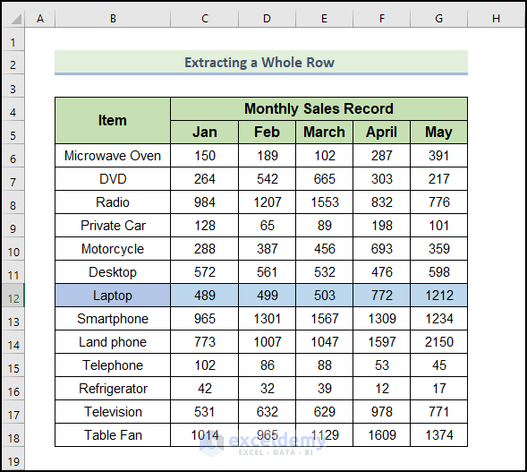
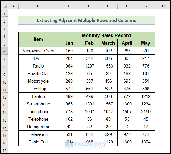
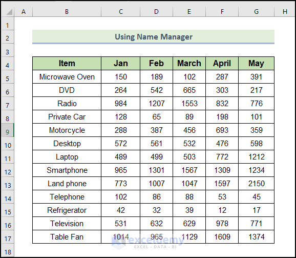
Here, we will demonstrate how to extract a whole row from a dataset in Excel. Our Excel dataset will be introduced to give you a better idea of what we’re trying to accomplish in this article. We have a sales record of 5 months of 13 products of a company named ABC Company. Now we will try to sort out a whole row using the OFFSET function. Let’s try to extract the sales record for laptop for all the months.
📌 Steps:
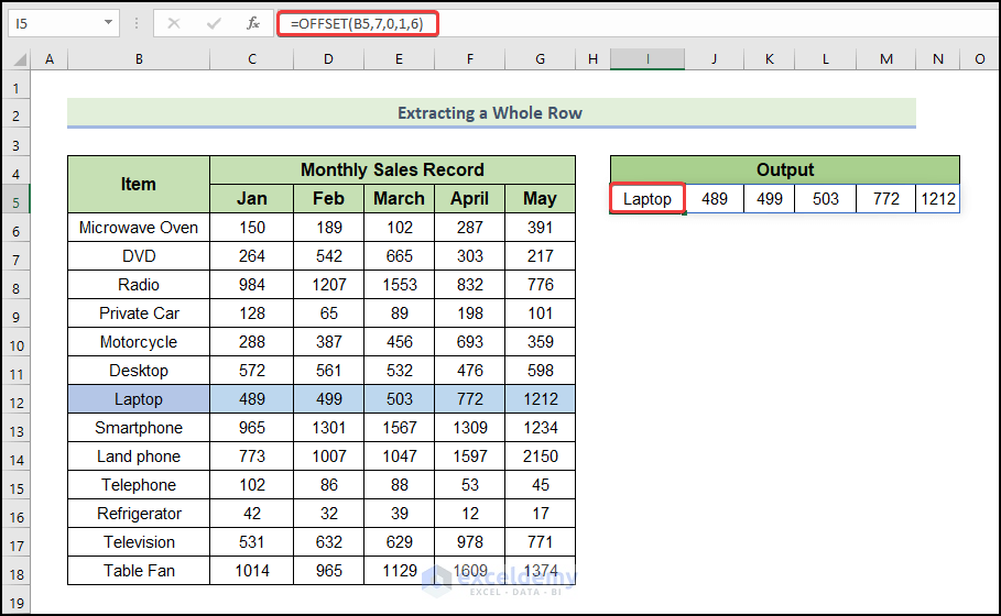
- To begin, type the following formula to extract the sales records for laptop for all the months.
=OFFSET(B5,7,0,1,6)
The OFFSET function starts moving from cell B5. Then it moves 7 rows downward to find the laptop. And then it extracts out a section of 1-row height and 6 columns of width. This is the sales record of laptop from Jan to May.
- Then, press Enter.
- Therefore, the output will look like this.
Read More: How to Use ROW Function in Excel (With 8 Examples)
2. Extracting an Entire Column
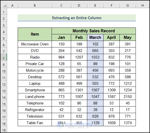
Now we’ll sort out a whole column from the same set of data. Let’s try to find out all the sales in March. And we will extract a list of a total of 13 products. Let’s walk through the following process to sort out a whole column from the dataset.
📌 Steps:
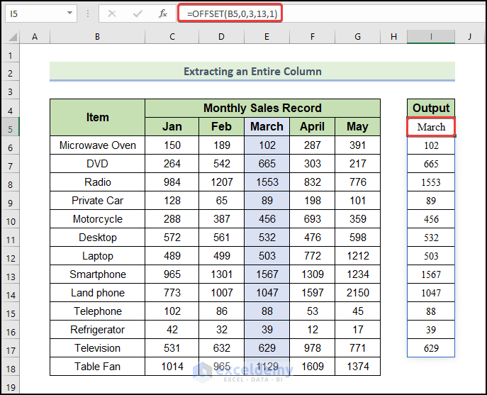
- First, type the following formula to sort out a whole column from the dataset.
=OFFSET(B5,0,3,13,1)
The function starts moving from cell B5. Moves 1 row down. Then move 3 columns right to the month of March. Then it extracts a section of 13 rows in height (all the products) and 1 column in width (only for the month of March).
- Then, press Enter.
- Therefore, the output will look like this.
Read More: How to Use COLUMN Function in Excel (4 Easy Examples)
3. Extracting Adjacent Multiple Rows and Columns
Now we will collect a section of multiple rows and multiple columns from the data set. Let’s try to collect the sales of the products Mototorcyle, Desktop, and Laptop in the months of January and February. Let’s walk through the following process to sort out adjacent multiple rows and columns from the dataset.
📌 Steps:
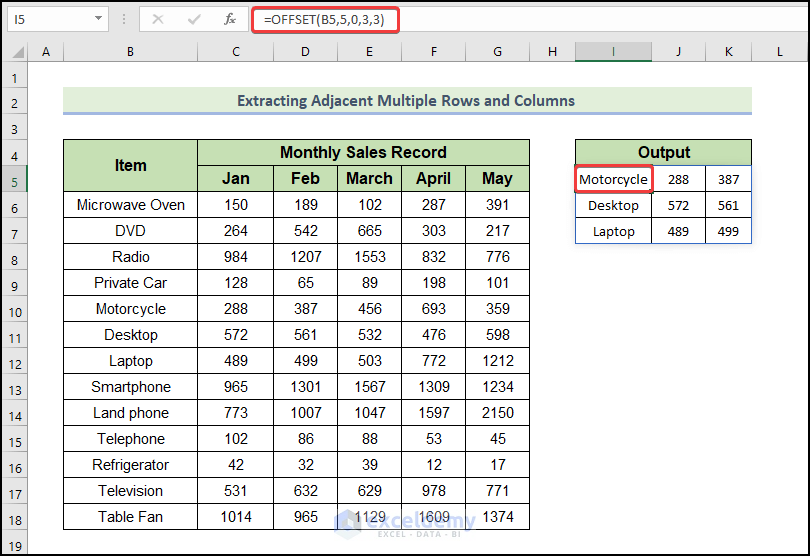
- First, type the following formula to sort out adjacent multiple rows and columns from the dataset.
=OFFSET(B5,5,0,3,3)
The function starts moving from cell B5. Then it moves 5 rows down to the product telephone. Then collects the data of 3 rows height.
- Then, press Enter.
- Therefore, the output will look like this.
Read More: How to Use ROWS Function in Excel (With 7 Easy Examples)
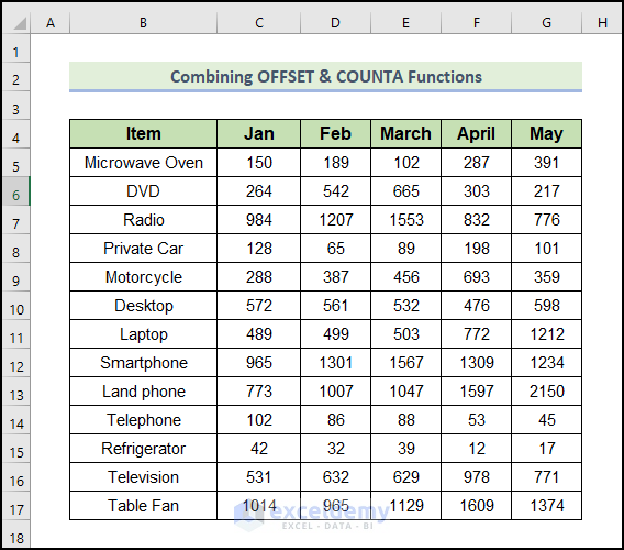
4. Combining OFFSET & COUNTA Functions to Create Dynamic Range
Here, we will show how to create a dynamic range with OFFSET and COUNTA functions. COUNTA function counts the number of cells excluding all empty cells in a range of cells. Now, using COUNTA functions, we’ll assign the row height & column width based on the available data in the range. Let’s walk through the following process to create a dynamic range with OFFSET and COUNTA functions.
📌 Steps:
- First, type the following formula.
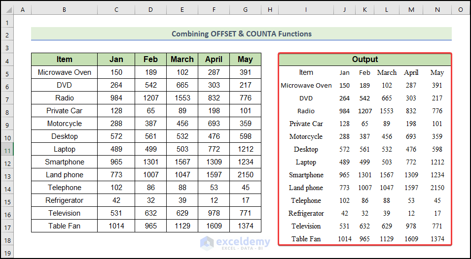
=OFFSET(B4,0,0,COUNTA(B4:B100),COUNTA(B4:G4))
Row height has been assigned with COUNTA(B4:B100) in the argument section, which means that each row in the spreadsheet is assigned up to the 100th row. This way, whenever a new value is entered under the original range of data within the 100th row, that value will also be stored using the OFFSET function. COUNTA(B4:G4) has been defined as the column width, so the six columns (B, C, D, E, F and G) are now assigned to the function based on the reference value selected in the OFFSET function.
- Then, press Enter.
- Therefore, the output will look like this.
5. Creating Dynamic Range Using Name Manager with OFFSET Function
By using Name Manager, you can set the name of the resultant array found by the OFFSET function. Let’s walk through the following steps to create a dynamic range using name manager.
📌 Steps:
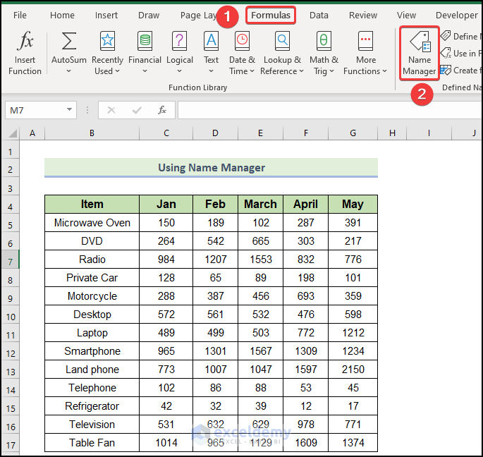
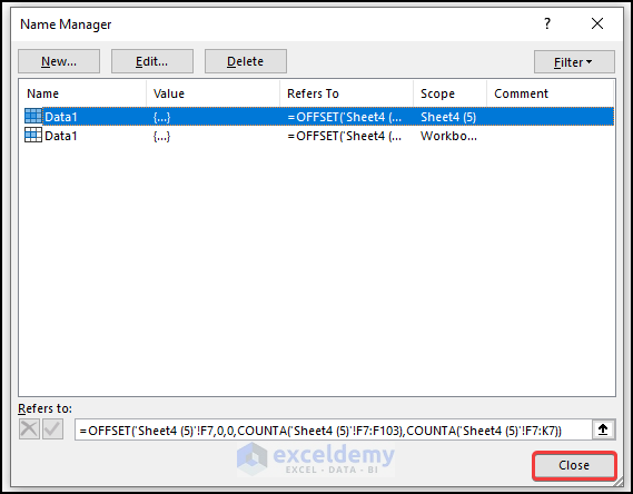
- First of all, under the Formula tab, select Name Manager.
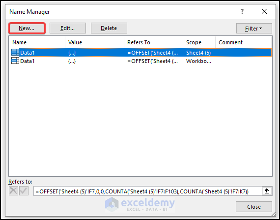
- A dialogue box will open.
- Then, press New.
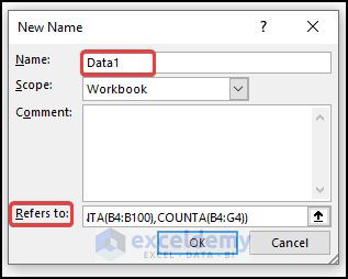
- Therefore, the Name Editor box will appear.
- Next, define the name of your dataset or the range of cells you want to offset.
- Afterward, in the reference box, type the formula:
=OFFSET(B4,0,0,COUNTA(B4:B100),COUNTA(B4:G4))
- Next, press OK & Name Manager will now show the defined name in the list along with the reference formula at the bottom.
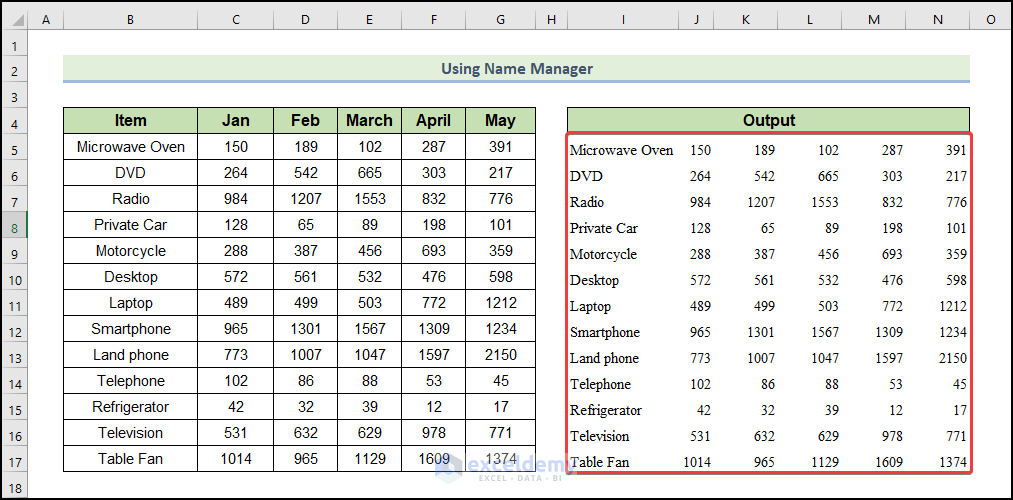
- Then, select any cell in your spreadsheet & start to type the defined name as the formula. You’ll find the defined name there in the function list.
- Next, select that function & press Enter.
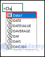
- Therefore, the output will look like this.
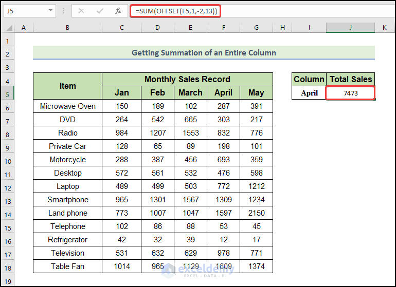
6. Getting Summation of an Entire Column
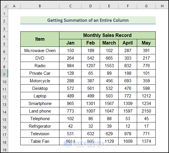
Here, we will demonstrate how to get the summation of an entire column by combining SUM and OFFSET functions in Excel. Let’s walk through the following steps to get the summation of an entire column.
📌 Steps:
- To begin, type the following formula in cell J5.
=SUM(OFFSET(F5,1,-2,13))
- Then, press Enter.
- Therefore, the output will look like this.
🔎 How Does the Formula Work?
- OFFSET(F5,1,-2,13)
The OFFSET function starts moving from cell F5. Then it moves 1 rows downward extracts teh records of sales of the April column.
- SUM(OFFSET(F5,1,-2,13))
The OFFSET function’s output will be summed by the SUM function.
Read More: How to use COLUMNS Function in Excel (3 Examples)
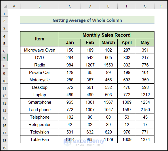
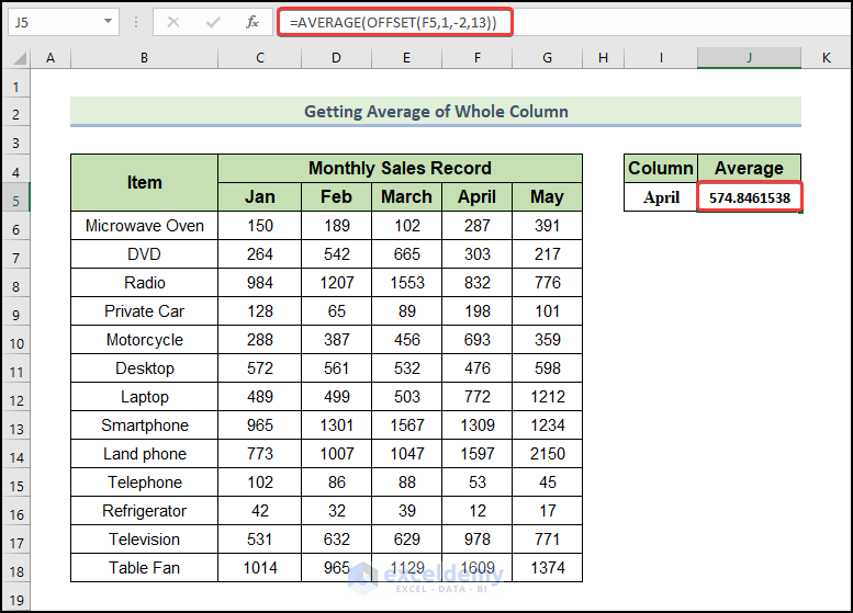
7. Getting Average of Whole Column
Here, we will demonstrate how to get the average of an entire column by combining AVERAGE and OFFSET functions in Excel. This is the last offset examples with formulas.Let’s walk through the following steps to get the average of an entire column.
📌 Steps:
- To begin, type the following formula in cell J5.
=AVERAGE(OFFSET(F5,1,-2,13))
- Then, press Enter.
- Therefore, the output will look like this.
🔎 How Does the Formula Work?
- OFFSET(F5,1,-2,13)
The OFFSET function starts moving from cell F5. Then it moves 1 rows downward extracts teh records of sales for the April column.
- AVERAGE(OFFSET(F5,1,-2,13))
In this case, we will use the AVERAGE function to average the output from the OFFSET function.
6 Suitable Examples of Offset Function with Excel VBA
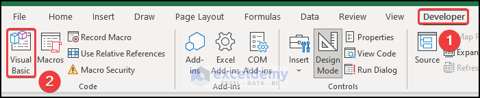
Below, we will examine five examples using VBA code that illustrate how to use the Excel OFFSET function. The following section provides detailed information about these examples. The following suggestions will help you improve your thinking capability and Excel knowledge. In this case, we’re using the Microsoft Office 365 version, but you can use any other version according to your preferences. If you want to write code in Excel, you need to use the help of VBA. Microsoft Visual Basic for Applications (VBA) is Microsoft’s Event Driven Programming Language. To use this feature you first need to have the Developer tab showing on your ribbon. Click here to see how you can show the Developer tab on your ribbon.
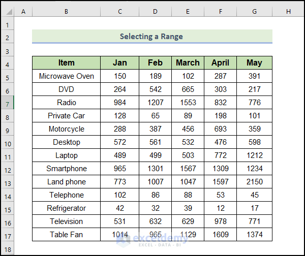
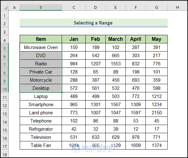
1. Selecting a Range
Here, we will demonstrate how to select a range in Excel. This is the first offset examples using VBA code. Let’s walk through the following steps to select range in Excel.
📌 Steps:
⧭ Open VBA Window:
- VBA has its own separate window to work with. You have to insert the code in this window too. To open the VBA window, go to the Developer tab on your ribbon. Then select Visual Basic from the Code group.
⧭ Insert Module:
- VBA modules hold the code in the Visual Basic Editor. It has a.bcf file extension. We can create or edit one easily through the VBA editor window. To insert a module for the code, go to the Insert tab on the VBA editor. Then click on Module from the drop-down.
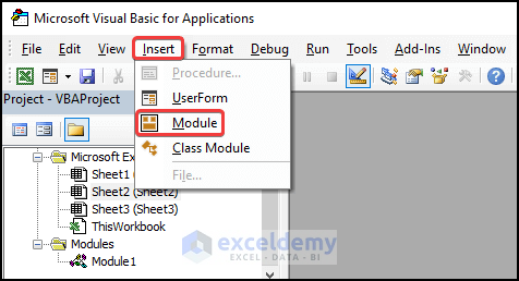
- As a result, a new module will be created.
⧭ Insert VBA Code:
- Now select the module if it isn’t already selected. Then write down the following code in it.
Sub selectrangeoffset()
Range("A1:A6").Offset(4, 1).Select
End Sub- Next, save the code.
⧭ Run VBA Code:
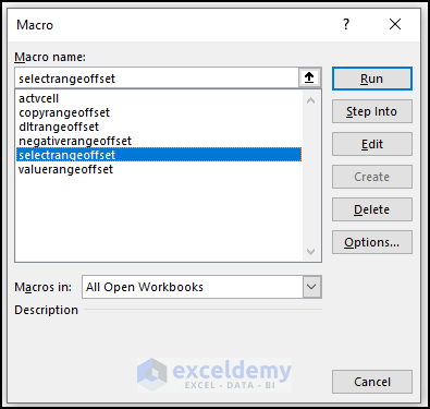
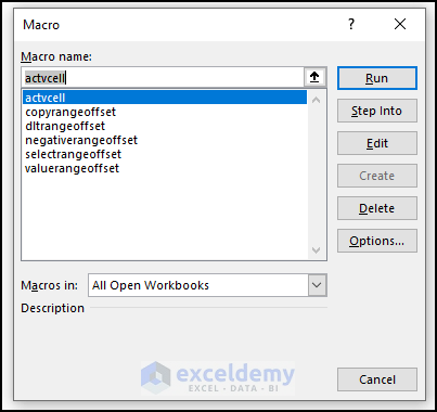
- Afterward, close the Visual Basic window. After that press Alt+F8.
- When the Macro dialogue box opens, select selectrangeoffset in the Macro name. Click on Run.
⧭ Output:
- Therefore, you will get the following output.
🔎 VBA Code Explanation:
Sub selectrangeoffset()First of all, provide a name for the sub-procedure of the macro.
Range("A1:A6").Offset(4, 1).SelectAt first, Range(“A1:A6”) will select the range A1:A6, and then Offset(4, 1) will move 4 rows downward from cell A1 and 1 column to the right side. After that, the equal number of cells in the range A1:A6 will be selected from here.
End SubFinally, end the sub-procedure of the macro.
2. Using Negative Value in Offset Property
Here, we will illustrate how to select negative value in Excel. To select negative values in Excel, follow these steps.
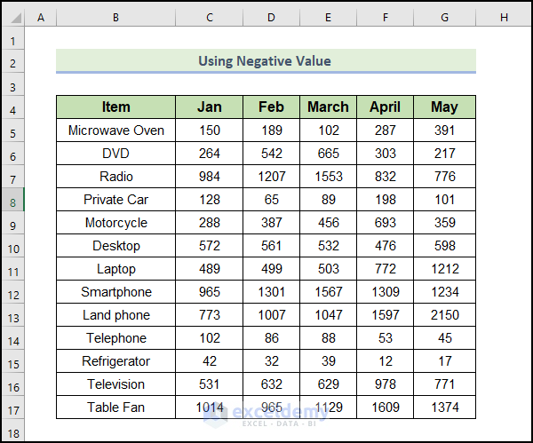
📌 Steps:
⧭ Open VBA Window:
- VBA has its own separate window to work with. You have to insert the code in this window too. To open the VBA window, go to the Developer tab on your ribbon. Then select Visual Basic from the Code group.
⧭ Insert Module:
- VBA modules hold the code in the Visual Basic Editor. It has a .bcf file extension. We can create or edit one easily through the VBA editor window. To insert a module for the code, go to the Insert tab on the VBA editor. Then click on Module from the drop-down.
- As a result, a new module will be created.
⧭ Insert VBA Code:
- Now select the module if it isn’t already selected. Then write down the following code in it.
Sub negativerangeoffset()
Range("F11:F16").Offset(-6, -2).Select
End Sub- Next, save the code.
⧭ Run VBA Code:
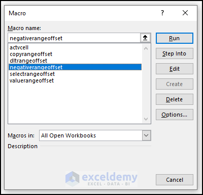
- Afterward, close the Visual Basic window. After that press Alt+F8.
- When the Macro dialogue box opens, select negativerangeoffset in the Macro name. Click on Run.
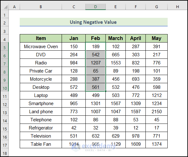
⧭ Output:
- Therefore, you will get the following output.
🔎 VBA Code Explanation:
Sub negativerangeoffset()First of all, provide a name for the sub-procedure of the macro.
Range("F11:F16").Offset(-6, -2).SelectAt first, Range(“F11:F16”) will select the range F11:F16, and then Offset(-6, -2) will move 6 rows upward from cell F11 and 2 columns to the left side. After that, the equal number of cells in the range D5:D10 will be selected from here.
End SubFinally, end the sub-procedure of the macro.
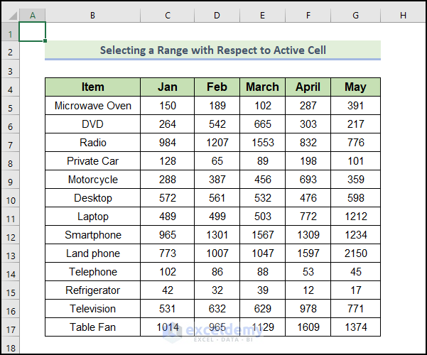
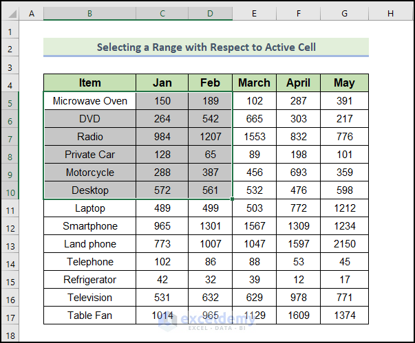
3. Selecting a Range with Respect to Active Cell
Here, we will illustrate how to select a range with respect to active cell in Excel. Let’s walk through the following steps to do the task in Excel.
📌 Steps:
⧭ Open VBA Window:
- VBA has its own separate window to work with. You have to insert the code in this window too. To open the VBA window, go to the Developer tab on your ribbon. Then select Visual Basic from the Code group.
⧭ Insert Module:
- VBA modules hold the code in the Visual Basic Editor. It has a.bcf file extension. We can create or edit one easily through the VBA editor window. To insert a module for the code, go to the Insert tab on the VBA editor. Then click on Module from the drop-down.
- As a result, a new module will be created.
⧭ Insert VBA Code:
- Now select the module if it isn’t already selected. Then write down the following code in it.
Sub actvcell()
Range(activecell.Offset(4, 1), activecell.Offset(9, 3)).Select
End Sub- Next, save the code.
⧭ Run VBA Code:
- Afterward, close the Visual Basic window. After that press Alt+F8.
- When the Macro dialogue box opens, select actvcell in the Macro name. Click on Run.
⧭ Output:
- Therefore, you will get the following output.
🔎 VBA Code Explanation:
Sub actvcell()First of all, provide a name for the sub-procedure of the macro.
Range(activecell.Offset(4, 1), activecell.Offset(9, 3)).SelectHere, activecell is A1. The first part activecell.Offset(4, 1) will select a cell 4 rows downward and 1 column right from the cell A1 and the second part activecell.Offset(9, 3) will select a cell 9 rows downward and 3 columns right from cell A1.
Finally, all of the cells between these two cells will be selected.
End SubFinally, end the sub-procedure of the macro.
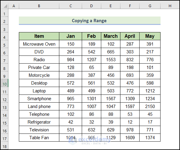
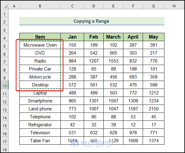
4. Copying a Range
Here, we will illustrate how to copy a range in Excel. We’ll walk through the steps to create a range in Excel by following the steps below.
📌 Steps:
⧭ Open VBA Window:
- VBA has its own separate window to work with. You have to insert the code in this window too. To open the VBA window, go to the Developer tab on your ribbon. Then select Visual Basic from the Code group.
⧭ Insert Module:
- VBA modules hold the code in the Visual Basic Editor. It has a.bcf file extension. We can create or edit one easily through the VBA editor window. To insert a module for the code, go to the Insert tab on the VBA editor. Then click on Module from the drop-down.
- As a result, a new module will be created.
⧭ Insert VBA Code:
- Now select the module if it isn’t already selected. Then write down the following code in it.
Sub copyrangeoffset()
Range("A1:A6").Offset(4, 1).Copy
End Sub- Next, save the code.
⧭ Run VBA Code:
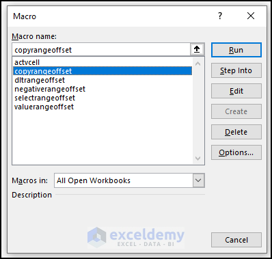
- Afterward, close the Visual Basic window. After that press Alt+F8.
- When the Macro dialogue box opens, select copyrangeoffset in the Macro name. Click on Run.
⧭ Output:
- Therefore, you will get the following output.
🔎 VBA Code Explanation:
Sub copyrangeoffset()First of all, provide a name for the sub-procedure of the macro.
Range("A1:A6").Offset(4, 1).CopyAt first, Range(“A1:A6”) will select the range A1:A6, and then Offset(4, 1) will move 4 rows downward from cell A1 and 1 column to the right side. After that, the equal number of cells in the range B5:B10 will be selected from here.
Finally, it will copy the values in the range B5:B10.
End SubFinally, end the sub-procedure of the macro.
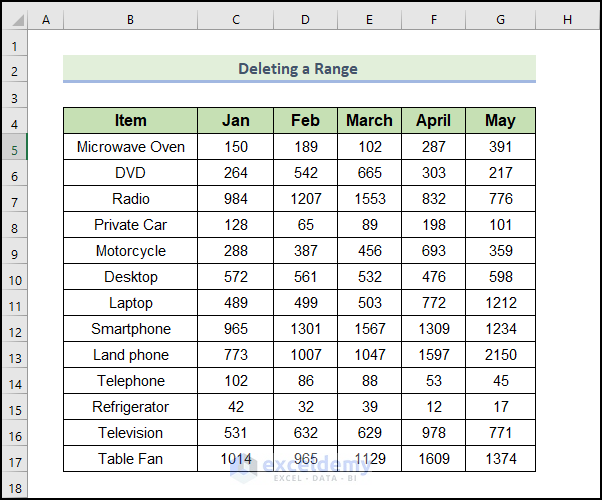
5. Deleting a Range
Here, we will demonstrate how to delete a range in Excel. Let’s walk through the following steps to delete a range in Excel.
📌 Steps:
⧭ Open VBA Window:
- VBA has its own separate window to work with. You have to insert the code in this window too. To open the VBA window, go to the Developer tab on your ribbon. Then select Visual Basic from the Code group.
⧭ Insert Module:
- VBA modules hold the code in the Visual Basic Editor. It has a.bcf file extension. We can create or edit one easily through the VBA editor window. To insert a module for the code, go to the Insert tab on the VBA editor. Then click on Module from the drop-down.
- As a result, a new module will be created.
⧭ Insert VBA Code:
- Now select the module if it isn’t already selected. Then write down the following code in it.
Sub dltrangeoffset()
Range("F11:F17").Offset(-7, -2).Delete
End Sub- Next, save the code.
⧭ Run VBA Code:
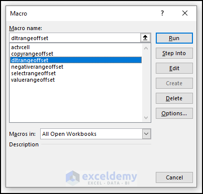
- Afterward, close the Visual Basic window. After that press Alt+F8.
- When the Macro dialogue box opens, select dltrangeoffset in the Macro name. Click on Run.
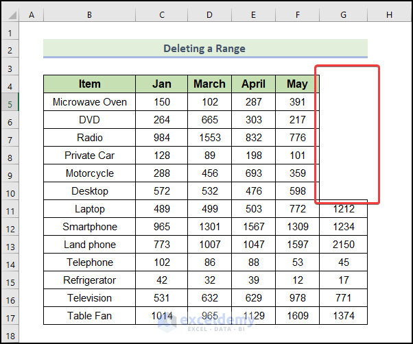
⧭ Output:
- Therefore, you will get the following output.
🔎 VBA Code Explanation:
Sub dltrangeoffset()First of all, provide a name for the sub-procedure of the macro.
Range("F11:F17").Offset(-7, -2).DeleteFirstly, Range(“F11:F17”) will select the range F11:F17, and then Offset(-7, -2) will move 7 rows upward from cell F11 and 2 columns to the left side. After that, the equal number of cells in the range G4:G10 will be selected from here.
Finally, it will delete the range G4:G10.
End SubFinally, end the sub-procedure of the macro.
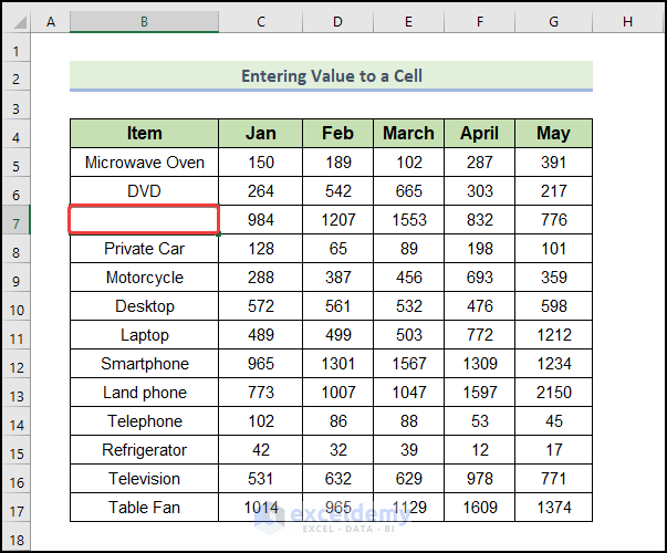
6. Entering Value to a Cell
Here, we will illustrate how to enter a value to a cell in Excel. This is the last example of “Excel offset function use with examples”. Here are the steps to do the task in Excel.
📌 Steps:
⧭ Open VBA Window:
- VBA has its own separate window to work with. You have to insert the code in this window too. To open the VBA window, go to the Developer tab on your ribbon. Then select Visual Basic from the Code group.
⧭ Insert Module:
- VBA modules hold the code in the Visual Basic Editor. It has a.bcf file extension. We can create or edit one easily through the VBA editor window. To insert a module for the code, go to the Insert tab on the VBA editor. Then click on Module from the drop-down.
- As a result, a new module will be created.
⧭ Insert VBA Code:
- Now select the module if it isn’t already selected. Then write down the following code in it.
Sub valuerangeoffset()
Range("A1").Offset(6, 1).Value = "Laptop"
End Sub- Next, save the code.
⧭ Run VBA Code:
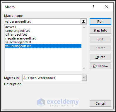
- Afterward, close the Visual Basic window. After that press Alt+F8.
- When the Macro dialogue box opens, select valuerangeoffset in the Macro name. Click on Run.
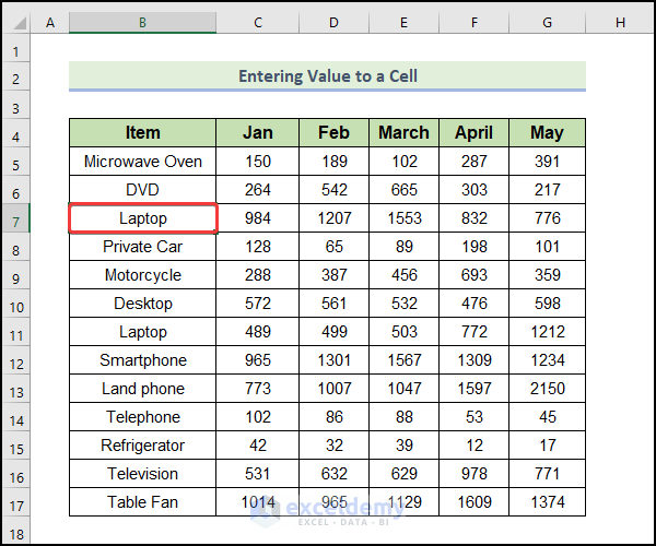
⧭ Output:
- Therefore, you will get the following output.
🔎 VBA Code Explanation:
Sub valuerangeoffset()First of all, provide a name for the sub-procedure of the macro.
Range("A1").Offset(6, 1).Value = "Laptop"Firstly, Range(“A1”) will select the cell A1, and then Offset(6, 1) will move 6 rows downward from cell A1 and 1 column to the right side. After that, cell B7 will be selected and finally, it will enter the value “Laptop” in this cell.
End SubFinally, end the sub-procedure of the macro.
Conclusion
That’s the end of today’s session. I strongly believe that from now, you may learn how to use use OFFSET function with examples in Excel. If you have any queries or recommendations, please share them in the comments section below.
Don’t forget to check our website Exceldemy.com for various Excel-related problems and solutions. Keep learning new methods and keep growing!
Further Readings
- How to Use INDIRECT Function in Excel (12 Suitable Instances)
- Find text in an Excel range & return cell reference (3 ways)
- Excel Reference Cell in Another Sheet Dynamically

