The INDEX function is one of the top used 10 Excel functions. In this tutorial, you will get a complete idea of how the INDEX function works in Excel individually and with other Excel functions.
You will get the Excel INDEX function in two forms: Array Form and Reference Form.
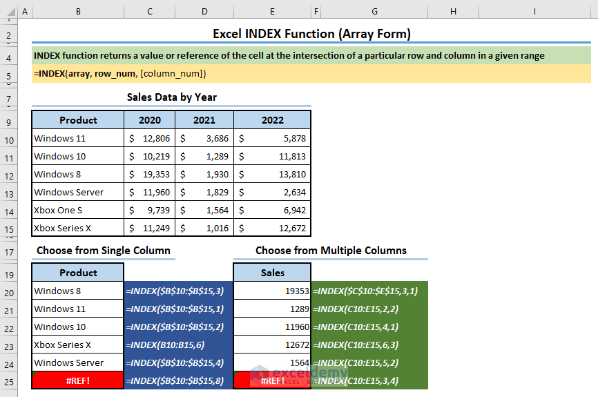
Excel INDEX Function in Array Form (Quick View):
When you intend to return a value (or values) from a single range, you will use the array form of the INDEX function.
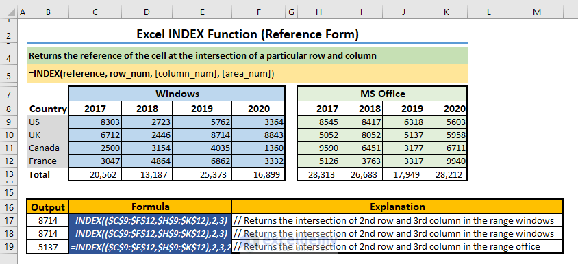
Excel INDEX Function in Reference Form (Quick View):
When you intend to return a value (or values) from multiple ranges, you will use the reference form of the INDEX function.
Introduction to INDEX Function in Excel
Function Objective:
It returns a value or reference of the cell at the intersection of a particular row and column, in a given range.
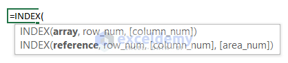
Syntax of INDEX Function in Array Form:
=INDEX (array, row_num, [column_num])
Arguments:
| argument | required/ optional | value |
|---|---|---|
| array | Required | Pass a range of cells, or an array constant to this argument |
| row_num | Required | Pass the row number in the cell range or the array constant |
| col_num | Optional | Pass the column number in the cell range or the array constant |
Note:
- If you use both the row_num and column_num arguments, the INDEX function will return the value from the cell at the intersection of the row_num and column_num.
- If you set row_num or column_num to 0 (zero), then you will get the whole column values or the whole row values respectively in the form of arrays. You can insert those values into cells using Array Formula.
Syntax of INDEX Function in Reference Form:
=INDEX (reference, row_num, [column_num], [area_num])
Arguments:
| argument | required/ optional | value |
|---|---|---|
| reference | Required | Pass more than one range or array |
| row_num | Required | Pass the row number in a specific cell range |
| col_num | Optional | Pass the column number in a specific cell range |
| area_num | Optional | Pass the area number that you want to select from a group of ranges |
Note:
- If pass more than one range or array as the array value, you should pass also the area_num.
- If the area_num is absent, the INDEX Function will work with the first range. If you pass a value as the area_num, the INDEX function will work in that specific range.
- If the concepts are not clear, do not worry; go to the next step, where I am going to show you a good number of examples to use Excel’s INDEX function effectively.
How to Use INDEX Function in Excel: 6 Handy Examples
Example 1: Select an Item from a List
Using the Excel INDEX function, we can retrieve any item from a list. You can use hard-coded row or column numbers in the formula or use a cell reference.
One Dimensional List with a Single Column:
For example, if we want to retrieve the 3rd product from the list, we can use the following formula in cell C13, having specified the row number (the serial number, in other words) in cell C12.
=INDEX(B5:B10,C12)Or,
=INDEX(B5:B10,3)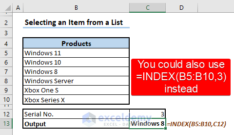
One Dimensional List with a Single Row:
Similarly, we can retrieve an item from a single row using the INDEX function. Specify the serial number in column B and apply the following formula in cell C20:
=INDEX(C17:H17,,B20)Or,
=INDEX(C17:H17,3)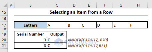
You could also write the serial number directly in the formula instead of using cell reference. But we recommend using cell reference as it makes your job more dynamic.
Retrieve Item from a Multidimensional List:
To retrieve an item from a list of multiple dimensions, you have to specify the row and column number in the INDEX function.
For example, If you want to get the item from the 3rd row and 4th column of the list, you must insert the following formula in cell C33.
=INDEX(C26:H29,C31,C32)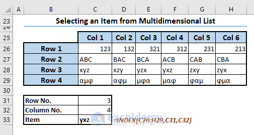
Note:
- If you specify a row number beyond the range of your list (the array you have specified to the INDEX function), it will cause a #REF! error.
- You can also refer to an array as a reference and apply the INDEX function. For example, the formula =INDEX({1,2,3;4,5,6;7,8,9;10,11,12},2,3) will return 8. The array constant {1,2,3;4,5,6;7,8,9;10,11,12} contains columns separated by semicolons.
Example 2: Selecting Item from Multiple Lists
You may have noticed already; that the INDEX function has another optional argument which is [area_num]. With this, you can input multiple arrays or reference ranges in the INDEX function and specify from which array, the function will return an item or value.
For example, we have two lists here, one is for Windows and the other is for MS Office. You can apply the following formula to get a value from the Windows list.
=INDEX((D5:G9,I5:L9),C11,E11,1)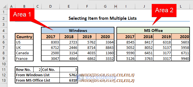
Or,
=INDEX((D5:G9,I5:L9),C11,E11,2)to get an item from the MS Office list.
Note:
If you don’t specify the number in this formula, Excel will consider area 1 to return the value, by default.
Example 3: Combine MATCH Function with INDEX to Match Multiple Criteria and Return Value
The MATCH function returns the relative position of an item in an array that matches a specified value in a specified order. You can easily retrieve the row and column numbers for a specific range using the MATCH function.
Let’s see the following example. We want to match some criteria specified in cells C12 and C13.
Steps:
- Apply the following formula in Cell C14:
=INDEX(B5:E10,MATCH(C13,B5:B10,0),MATCH(C12,B4:E4,0))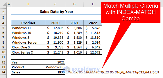
- Press ENTER.
🔎 How Does This Formula Work?
Let’s see how this formula works part by part.
- MATCH(C12,B4:E4,0)
Output: 3
Explanation: The MATCH function takes input from cell C12 and performs an exact match in the range B4:E4. 0 digit in the last argument indicates an exact match here. Finally, since the item in C12 is in the third column of the B4:E4 range, the function returns 3.
- MATCH(C13,B5:B10,0)
Output: 3
Explanation: Same as the first MATCH function explained above. But this time, the function works row-wise since the range B5:B10, which means the items are in different rows but in one single column.
- INDEX(B5:E10,MATCH(C13,B5:B10,0),MATCH(C12,B4:E4,0))
Output:1930
Explanation: We can simplify the formula using the outputs of the two MATCH parts. So it will be INDEX(B5:E10,3,3). So, the INDEX function will travel to row 3 and then to column 3 within the range B5:E10. From the row-column intersection, it will return that value.
Example 4: Combine INDEX, MATCH, and IF Functions to Match Multiple Criteria from Two Lists
Now, if we have two lists and want to match multiple criteria after choosing one, what to do? Here, we will provide you with a formula.
Here is our dataset and we have Sales data for Windows and MS Office in different countries and years.
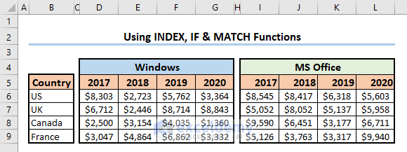
We will set 3 criteria: Product name, Year, and Country, and retrieve their corresponding sales data.
Steps:
- Assume that the criteria set are- Year: 2019, Product: MS Office, and Country: Canada.
- Set them in cells C11, C12, and C13 respectively.
- Now, apply the following formula in Cell C14 and hit ENTER.
=INDEX(INDEX((D5:G9,I5:L9),,,IF(C12="Windows",1,2)),MATCH(C13,B5:B9,0),MATCH(C11,INDEX((D5:G5,I5:L5),,,IF(C12="Windows",1,2)),0))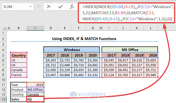
- You will see the corresponding sales data in Cell C14 now.
- You can make this formula more dynamic by using data validation.
🔎 How Does This Formula Work?
- IF(C12=”Windows”,1,2))
Output: 2
Explanation: Since Cell C12 contains Windows, the criteria is not matched and the IF function returns 2.
- INDEX((D5:G9,I5:L9),,,IF(C12=”Windows”,1,2))
Output: {2017,2018,2019,2020;8545,8417,6318,5603;5052,8052,5137,5958;9590,6451,3177,6711;5126,3763,3317,9940}
Explanation: Since the IF(C12=”Windows”,1,2) part returns 2, so this formula becomes INDEX((D5:G9,I5:L9),,,2). Now, the INDEX function returns the second range assigned to it.
- MATCH(C11,INDEX((D5:G5,I5:L5),,,IF(C12=”Windows”,1,2)),0)
Output: 3
Explanation: Since IF(C12=”Windows”,1,2) part returns 2, so this part becomes MATCH(C11,INDEX((D5:G5,I5:L5),,,2),0). Now, INDEX((D5:G5,I5:L5),,,2) part return I5:G5 which is {2017,2018,2019,2020}. So the MATCH formula becomes MATCH(C11,{2017,2018,2019,2020},0). And the MATCH function returns 3 since the value 2019 in Cell C11 is in the 3rd position of {2017,2018,2019,2020} array.
- MATCH(C13,B5:B9,0),
Output: 4
Explanation: The MATCH function matches the value of Cell C13 in the B5:B9 range and returns 4 since it’s the position of the string “Canada” in the B5:B9 range.
- =INDEX({2017,2018,2019,2020;8545,8417,6318,5603;5052,8052,5137,5958;9590,6451,3177,6711;5126,3763,3317,9940},4,3)
Output: 3177
Explanation: After all the small pieces of the formula are performed, the whole formula looks like this. And it returns the value where the 4th row and 3rd column intersect.
Example 5: Returning a Row or Column Entirely from a Range
Using the INDEX function, You can also return a row or column entirely from a range. To do that, execute the following steps.
Steps:
- Say you want to return the first row from the Windows list. Apply the following formula in any cell (here, in cell F11), and press ENTER.
=INDEX(D6:G9,1,0)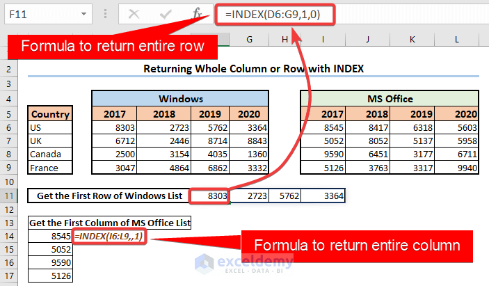
- Note that, we have specified the column number as 0 here. We could also apply the following formula to get the entire row, putting a comma after the row_num argument, and leaving it as it is without specifying any column number.
=INDEX(D6:G9,1,)- But if you just write =INDEX(D6:G9,1) and hit ENTER, you will get only the first value in the first row, not the whole row.
- To get the first column as a whole, apply the following formula. The things you should consider in case of getting a whole row returned are also applicable to this case.
=INDEX(I6:L9,,1)Note:
- If you are using older Excel versions than Microsoft 365, then you must use the Array formula to return a row or column from a range using the INDEX Function.
- For example, in our dataset here, every row of the sales range consists of 4 values, so you must select 4 cells horizontally and then input the INDEX function.
- Now press CTRL + SHIFT + ENTER to enter the formula as an array formula.
- In the same way, you can show the Entire Column.
- To return an entire range, just assign the range to the reference argument and put 0 as the column and row number. Here is a formula as an example.
=INDEX(D6:G9,0,0)Example 6: INDEX Function Can Also Be Used as Cell Reference
In example 5, we have seen how to use the INDEX function to return an entire row from a range. You could also use the following simple formula in any cell to get the same.
=D6:G6The point I am trying to make is- the INDEX function can also return a cell reference instead of a cell value. I will use INDEX(D6:G9,1,4) instead of G6 in the above formula. Hence, the formula will be like this,
=D6:INDEX(D6:G9,1,4)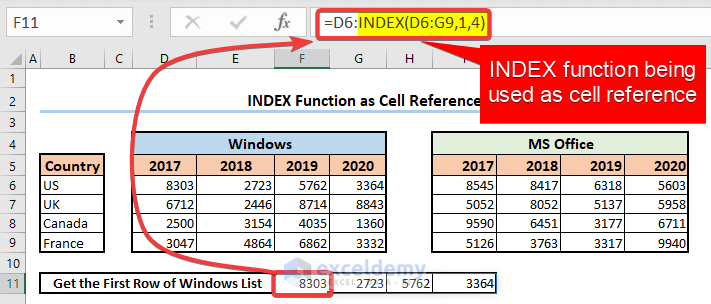
🔎 Evaluation of This Formula:
- First, select the cell where the formula lies.
- Go to the Formulas tab >> Formula Auditing group >> Click on the Evaluate Formula command.
- The Evaluate Formula dialog box will open.
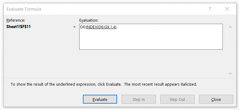
- In the Evaluation field, you will get the formula =D6:INDEX(D6:G9,1,4).
- Now click on Evaluate.
- The formula is now showing the cell range $D$6:$G$6.
- So, the whole INDEX formula has returned a cell reference, not a cell value.
What Are the Common Errors While Using the INDEX Function in Excel?
The #REF! Error:
It occurs-
- When your passed row_num argument is higher than the existing row numbers in the range.
- When your passed col_num argument is higher than the existing column numbers in the range.
- When your passed area_num argument is higher than the existing area numbers.
The #VALUE! Error:
It occurs when you supply non-numeric values as row_num, col_num, or area_num.
Download Excel Workbook
Download the Excel workbook so that you can practice yourself.
Conclusion
INDEX Function is one of the most powerful functions in Excel. To travel through a range of cells, and retrieve data from a range of cells, you will use a lot of time Excel’s INDEX Function. If you know a unique way of using Excel’s INDEX Function, let us know in the comment box.
<< Go Back to Excel Functions | Learn Excel
Get FREE Advanced Excel Exercises with Solutions!

Have tried the links to download the 1200+ macros examples e-book & 100+ excel functions cheat sheet. However, it keeps asking me to reload or re-register. Please if the file sizes are not too large can you forward to my email address.
Baber,
I have sent you an email with instructions. Please check. I hope the email solves the problem.
Regards
How about adding a link to save the content for later reference?
Ahmed Sheikh
[email protected]
You can do that Ahmed. Thank you.
Regards
I have many data in columns A to E , I want to find all data that corresponding to a specific data from column A . This data from A may be exist three times or more.
I have many data in columns A to E , I want to find all data from column E that corresponding to a specific data from column A. This data from A may be exist three times or more.
Waleed,
Can you upload the working files of your problems? At least a sample file? If possible send an email to this address [email protected]
I am trying to use the index function to display a dollar amount listed in a table in the month that it will be billed for. I have multiple projects and when the formula is dragged down to the next project, the index gets off because the projects have different start dates. Is there a better way to have the index start at the first billing month other than copying the formula from the previous project to the first billing month of the next project?
Hi, GILBERT BECHTOL!
Thank you for your query.
In your appeared problem, I would suggest you use the MONTH function to get individual months from each date record. Then, sort the order from smallest to largest. As a result, you’ll get the billing months of the project in sequential order and thus you can use the INDEX function to achieve your target.
If your problem still doesn’t fix, please send us your Excel sheet with clearer feedback on your target in this regard.
Regards,
Tanjim Reza
Dear All:
I am looking for a way (without VBA) to create a dynamic array constant which has the value of {1,1,1;2,2,0;3,0,0} in column 3 and {1,1,1,1;2,2,2,0;3,3,0,0;4,0,0,0} in column 4.. and so on and so forth
This is where I have reached so far:
I was able to figure out that an array formula =CHOOSE(TRANSPOSE(A1:C1),{1,1,1},{2,2,0},{3,0,0}) where A1=1,B1=2,C1=3 gives me the solution and =A1*–(A1:A3<D1) gives me the value of {1,1,1}.. but when I try combining the above two into a single formula as =CHOOSE(TRANSPOSE(A1:C1),A1:C1*–(OFFSET(A1:C1,0,0,1,C1)<D1)).. i am returned the value of {1,2,3;#VALUE!,#VALUE!,#VALUE!;#VALUE!,#VALUE!,#VALUE!}….
I cant seem to figure out how to get the above formula to work or some other way to get the constant {1,1,1;2,2,0;3,0,0}.
Please do help.
Thanks
Akshay
Hi AKSHAY THAKKER! We hope you are well. It’s been 6 years since you posted this query here. We are extremely sorry for being so late in responding. Hope you would have had a solution to your problem somewhere by now. However, we are providing a solution to your question hoping that other readers might find it useful.
For example, we have created a 10×10 array using the following formula.
Look at the following image.
You must do two things before applying the formula.
First, place the numbers in the first row (row 1, i.e. row of A1) serially, and second, place them serially down the first column (column A). You can place them elsewhere, but in that case, you have to change the cell references in the array formula accordingly.
You can create any square array with your desired sequence (1,1,1,1;2,2,2,0;3,3,0,0;4,0,0,0) having any square dimension. However, if you want to change the sequence, you have to change the formula a bit.
Tip: Look into the greater than logic in the formula. You have to make the change here to create other sequences.
If there is any query, please let us know. You can also send us your problem at this address: [email protected]