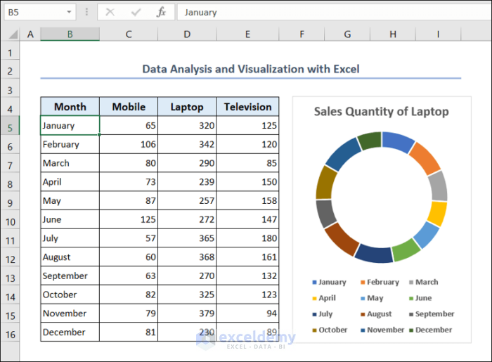
In this article, we will show you how to perform data analysis and visualization with Excel. There are three stages in data analysis and visualization. To begin, we will show you how to do data processing. Then, we will describe how to analyze data with various Excel features and functions. We will explore pivot tables, data sorting, data validation, and many more techniques. At the end, we will explore how to visualize data with different useful charts.
Data analysis and visualization with Excel is very significant for gaining valuable insights and understanding patterns and outliers of a dataset.
Download Practice Workbook
You can download this practice workbook while going through the article.
What is Data Analysis and Visualization?
Data Analysis is a process of collecting, organizing, and analyzing raw data to find relevant information. This information is vital to make data driven decisions. By doing data analysis, we can get valuable insights into the dataset and ensure accuracy in our decision making.
On the other hand, visualization is basically the graphical representation of the dataset. Different types of charts can help us to understand our data points and identify patterns, trends, and outliers of the dataset. Visualization makes our raw data more comprehensible and accessible.
Excel comes with many powerful features and functions for data analysis and visualization.
Steps of Data Analysis and Visualization with Excel
When it comes to data analysis and visualization with Excel, we will use the following steps.
1. Data Processing
2. Data Analysis
3. Data Visualization
We will explore these steps at length in the following sections.
1. Data Processing
In this section, we will learn about data processing. This is the first step of data analysis and visualization. It has the following segments.
1.1. Data Collection
First, you have to collect information. The information should be collected in a systematic way from a trustworthy source. The source can be any database, online platform, or any web page. Then this data needs to be further processed.
1.2. Data Organization
After collecting the data, the next step is to organize the data in such a way that it is easily understandable to people. The data can be arranged in a tabular form with a clear title and headings.
1.3. Data Cleaning
The organized data may require further cleaning. It may include blank spaces, unwanted empty cells, and duplicate values. So, data cleaning is basically making the dataset accurate and errorless.
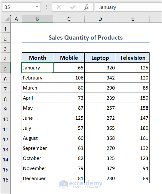
Here, we have processed our dataset accordingly. The dataset contains the sales quantity of products such as mobiles, laptops, and televisions of a company. The sales quantity is provided monthly basis. We will use this dataset for our data analysis and visualization with Excel.
2. Data Analysis
There are many techniques for data analysis in Excel. We will show you these techniques one by one.
2.1. Use Excel Functions
There are numerous functions available in Excel for data analysis. Let us walk you through some useful functions and their applications.
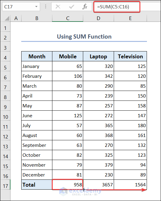
2.1.1. Use SUM Function
We can use the SUM function to find out the total number of mobile, laptop, and television sold in a year.
- Go to cell C17 and put the following formula.
=SUM(C5:C16)- Select cell C17 and use Fill Handle to AutoFill data in range D17:E17.
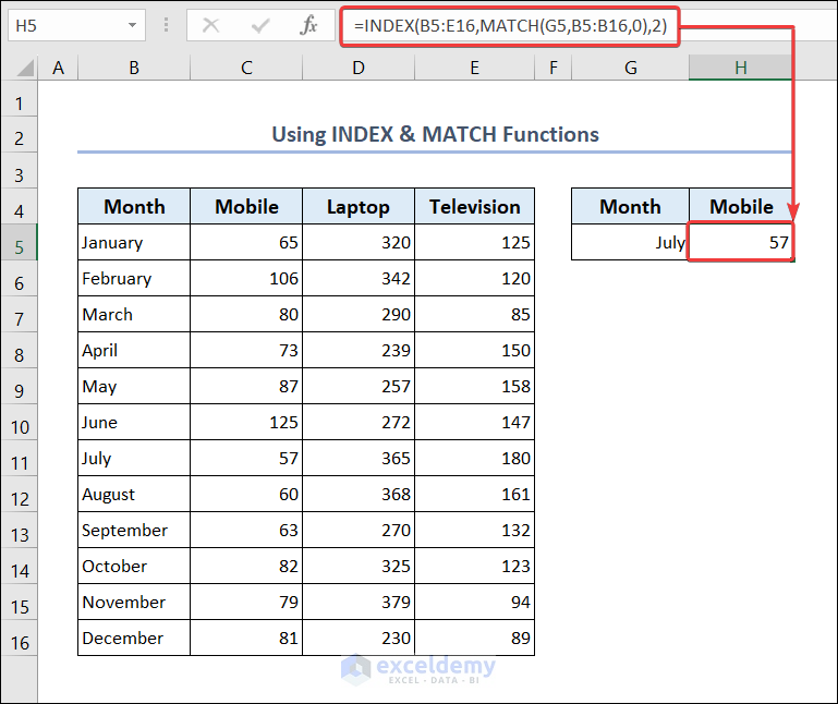
2.1.2. Use INDEX & MATCH Functions
You can use the combination of INDEX & MATCH functions to find out the sales quantity of a particular product for any month.
- Go to cell G5 and type the name of any month there.
- Go to cell H5 and put the following formula.
=INDEX(B5:E16,MATCH(G5,B5:B16,0),2)- You will see the sales quantity of mobiles for that particular month.
- You can change the month name in cell G5 and the sales quantity of mobile will be shown in cell H5.
Formula Breakdown
MATCH(G5,B5:B16,0): The MATCH function searches for the value of cell G5 within a specified range B5:B16. The 0 indicates that it must be an exact match.
Result: 7
INDEX(B5:E16,MATCH(G5,B5:B16,0),2): The INDEX function uses the row number returned by the MATCH function. It then returns value from the particular row number and the second column (2) of range B5:E16.
Result: 57
2.1.3. Use VLOOKUP & MATCH Functions
You can use the combination of VLOOKUP & MATCH functions to get the sales quantity of any product for any month.
- Go to cell H4 and put the name of any month there.
- Go to cell H5 and put the product name there.
- Go to cell H6 and put the following formula.
=VLOOKUP(H4,B5:E16,MATCH(H5,B4:E4,0))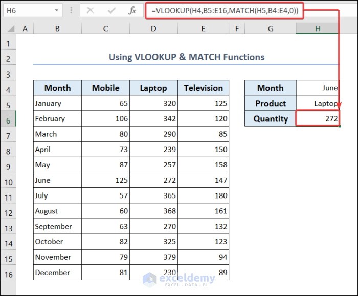
You can see the sales quantity of the product for the given month in cell H6.
Formula Breakdown
MATCH(H5,B4:E4,0): The MATCH function searches for the value of cell H5 within a specified range B4:E4. The 0 indicates that it must be an exact match.
Result: 3
VLOOKUP(H4,B5:E16,MATCH(H5,B4:E4,0)): The VLOOKUP function searches for the value of cell H4 in the leftmost column in the range B5:E16. Once it finds a match, it returns the value from the same row and the column specified by the MATCH function output.
Result: 272
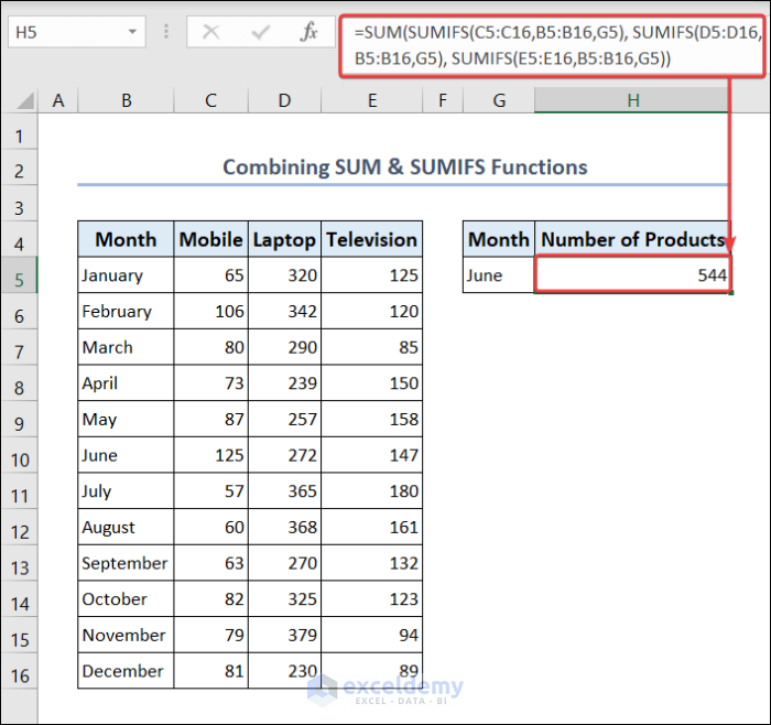
2.1.4. Combine SUM & SUMIFS Functions
We can combine the SUM & SUMIFS functions to get the number of products sold for any month.
- Go to cell G5 and put the name of the month.
- Go to cell H5 and put the following formula.
=SUM(SUMIFS(C5:C16,B5:B16,G5), SUMIFS(D5:D16,B5:B16,G5), SUMIFS(E5:E16,B5:B16,G5))- You will see the total number of products for that month.
Formula Breakdown
SUMIFS(C5:C16,B5:B16,G5): The SUMIFS function sums the value of range C5:C16 but it only includes those values where the corresponding cells of range B5:B16 match the value of cell G5.
Result: 125
SUMIFS(D5:D16,B5:B16,G5): The SUMIFS function sums the value of range D5:D16 but it only includes those values where the corresponding cells of range B5:B16 match the value of cell G5.
Result: 272
SUMIFS(E5:E16,B5:B16,G5): The SUMIFS function sums the value of range E5:E16 but it only includes those values where the corresponding cells of range B5:B16 match the value of cell G5.
Result: 147
SUM(SUMIFS(C5:C16,B5:B16,G5), SUMIFS(D5:D16,B5:B16,G5), SUMIFS(E5:E16,B5:B16,G5)): The SUM function adds the result of the three SUMIFS functions. It takes the sums of values in range C5:C16, range D5:D16, and range E5:E16, but only includes values where the corresponding cells in the range B5:B16 match the value in cell G5.
Result: 544
2.1.5. Apply MAX, INDEX & MATCH Functions
You can apply the MAX function to get the most quantity sold in a month for a particular product. Then you can use the INDEX & MATCH functions to find out the month in which the product was sold the most.
- Go to cell G6.
- Put the following formula to find the maximum number of laptops sold in a month.
=MAX(D5:D16)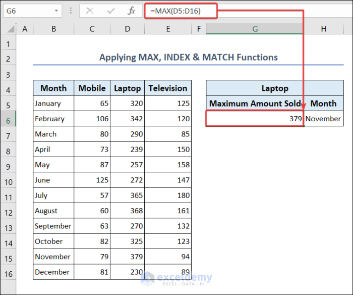
- Then go to cell H6.
- Put the following formula to find the name of that month.
=INDEX(B5:E16,MATCH(G6,D5:D16,0),1)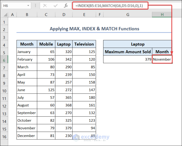
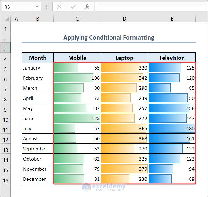
2.2. Apply Conditional Formatting
You can apply conditional formatting to understand the relative quantity of individual products sold over the span of 12 months.
- Select range C5:C16.
- Go to the Home tab >> select Conditional Formatting >> Data Bars.
- Now select any fill color to highlight the cells.
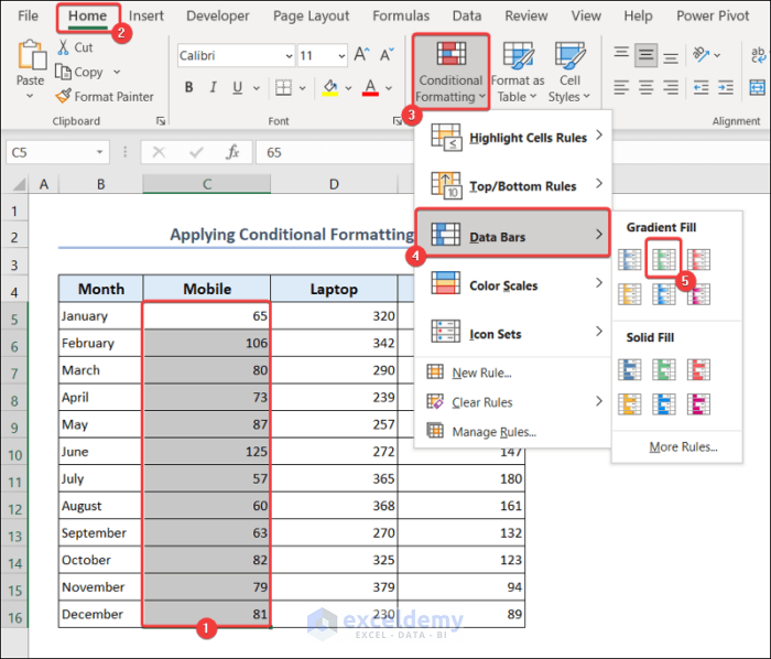
- Do the same steps for range D5:D16 and range E5:E16 as well.
2.3. Use Pivot Table
- Go to the Insert tab >> Pivot Table >> From Table/Range.
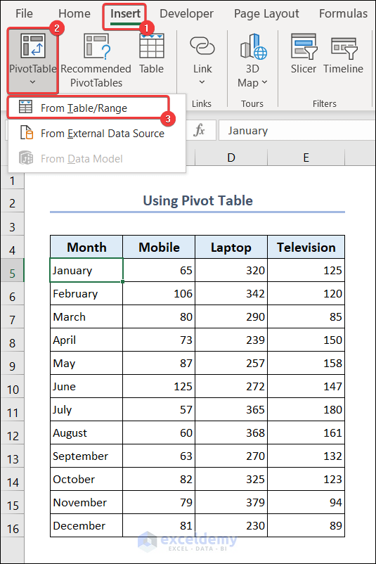
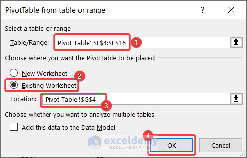
- A dialog box will appear. Set the dialog box as shown below.
- Put the following range as the Table/Range.
'Pivot Table'!$B$4:$E$16- Set location of the pivot table in cell G4 of the Existing Worksheet and press OK.
- Now set the PivotTable Fields as shown below. Drag the fields in different areas.
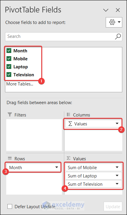
- You will have the pivot table with the grand total of the products.

2.4. Sort a Product
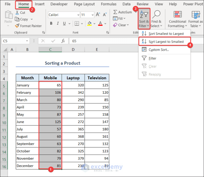
You can sort any product in ascending or descending order. We will sort the dataset in descending order with respect to the Mobile column.
- Select range C5:C16.
- Go to the Home tab >> Sort & Filter >> Sort Largest to Smallest.
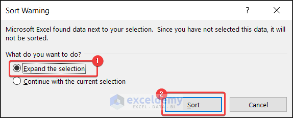
- Select Expand the selection >> press Sort.
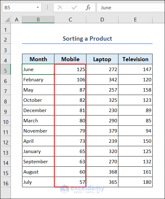
- The dataset will be sorted according to the sales quantity of mobile phones in descending order.
2.5. Filter Data
- Select range B4:E16.
- Go to the Home tab >> Sort & Filter >> Filter.
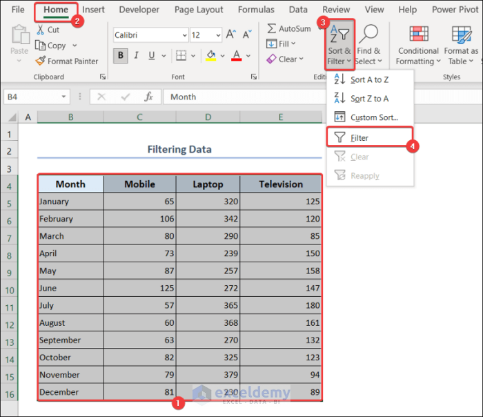
- You will have the filter icons in all the columns.
- Select the filter icon of the Month column.
- Choose the month you want to see and click on OK.
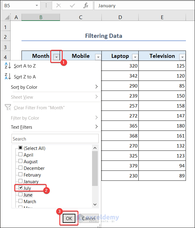
- You will see the filtered data of that month only.

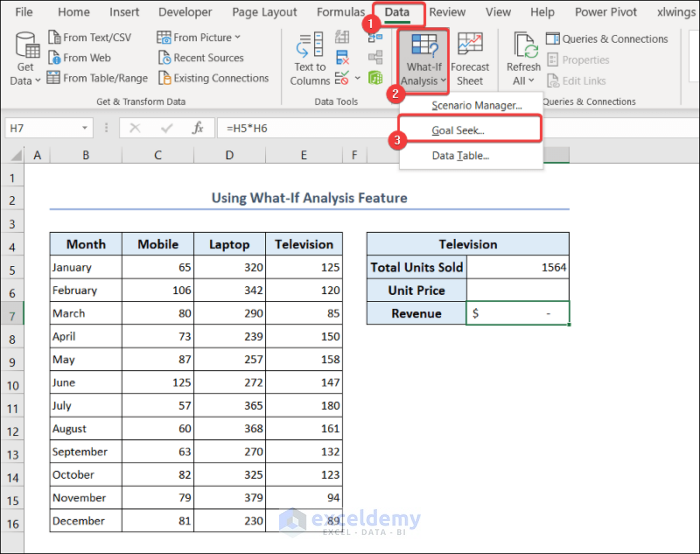
2.6. Use What-If Analysis Feature
Excel comes with a strong feature named What-If Analysis. It is a combination of techniques and tools that help you to predict the impact on the results of your formulas and models. It comes with the following features.
Goal Seek: This feature predicts the value of a parameter to achieve a specific output. You need to specify the target value and Excel will determine the input value in such a way that it reaches the desired outcome.
Scenario Manager: In this feature, you can define different scenarios for different inputs. You can switch between the inputs to see how the output varies.
Data Table: It allows you to create a table and evaluate multiple results based on input values. You can use these tables with one or two variables to see how different inputs affect the output.
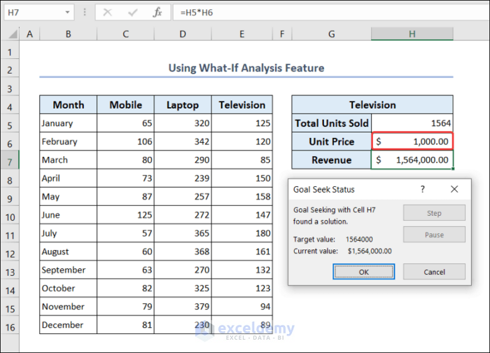
We will show you an example of the Goal Seek feature. The total units of television sold is 1564. We want to generate a revenue of $1564000. We will find the unit price of televisions required to reach this revenue.
- Put the following formula in cell H7.
=H5*H6- Go to the Data tab >> What-If Analysis >> Goal Seek.
- Set the Goal Seek dialog box as shown below.
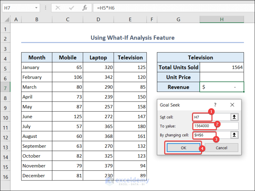
- You will get the unit price in cell H6 that is required to reach desired revenue which is $1564000.
2.7. Apply Data Validation
You can use data validation to choose any month from a given list. Here, we will find the sales quantity of laptops for any month.
- Select cell G5.
- Go to the Data tab >> select Data Validation.
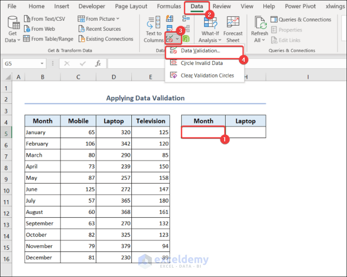
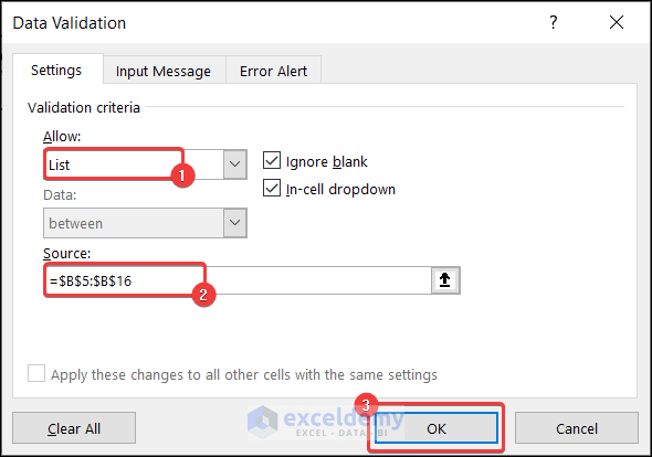
- Data Validation dialog box will appear.
- Choose List in the Validation criteria.
- Set Source location as follows.
=$B$5:$B$16- Press OK.
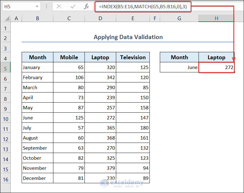
- You will have a dropdown in cell G5.
- Select any month from the dropdown list.

- Go to cell H5 and put the following formula.
=INDEX(B5:E16,MATCH(G5,B5:B16,0),3)- You will see the sales quantity of laptops for that month.
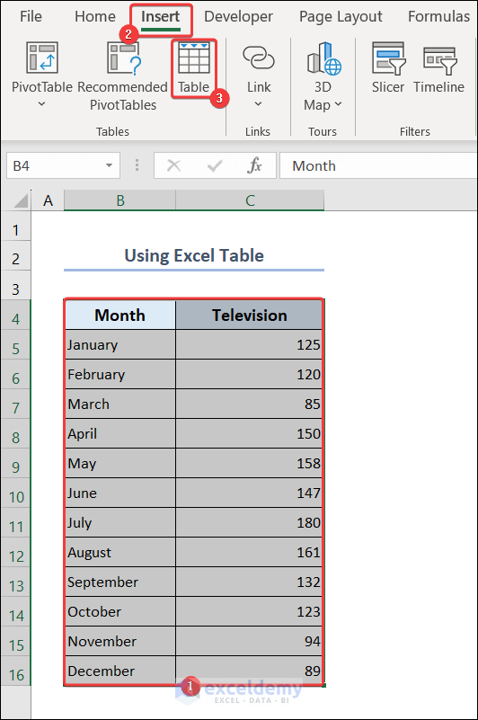
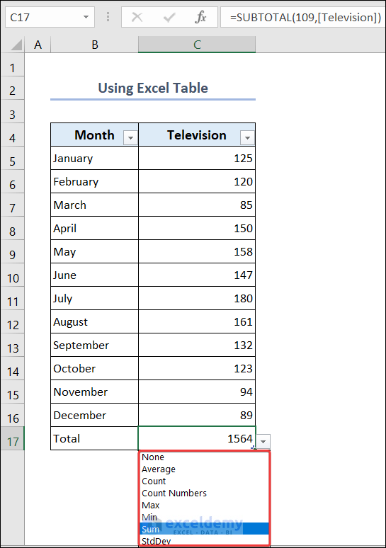
2.8. Use Excel Table
We can create a table to filter data, automate formulas and find parameters like sum, average, maximum, minimum, and so on.
- Select range B4:C16.
- Go to the Insert tab >> Table.
- Check the My table has headers option.
- Press OK.
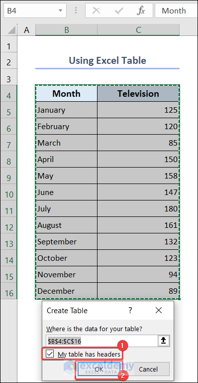
- The table will be created.
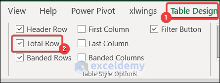
- Select Total Row from the Table Design tab.
- You will see the total number of televisions in cell C17.
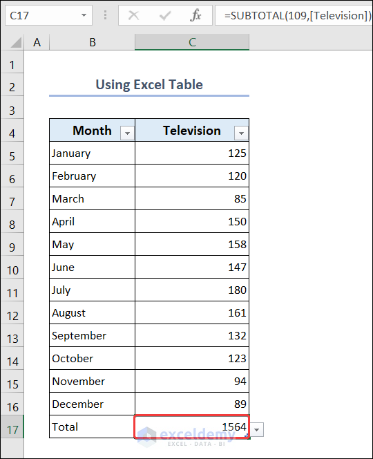
- You will also have a drop-down in cell C17. From there you can choose any parameter you want to see.
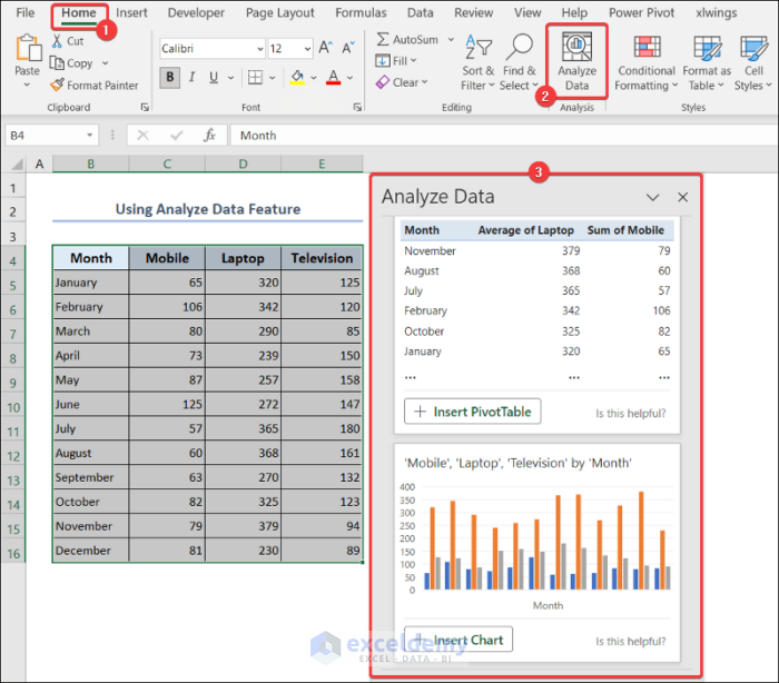
2.9. Use Analyze Data Feature
- Go to the Home tab >> Analyze Data.
- You will find different options like pivot tables and charts to analyze your dataset.
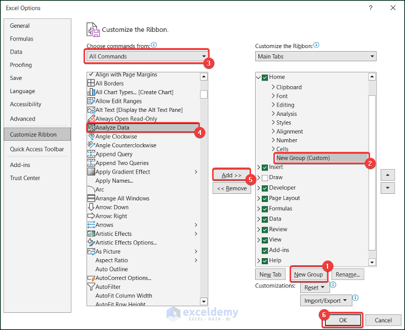
If you do not see the Analyze Data option in your Home tab, you have to customize it.
- Right-click on the Home tab >> select Customize Ribbon.
- Add a New Group >> set its position >> select All Commands >> find Analyze Data from the list >> Add this to the newly created group >> click OK.
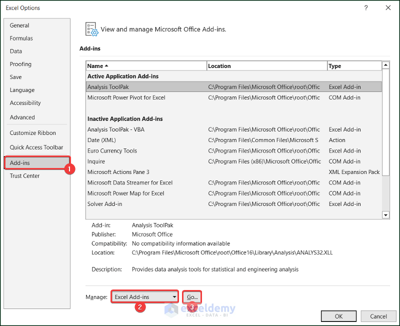
2.10. Use Analysis ToolPak Add-in
You can perform a wide range of analysis using the Analysis ToolPak add-in. Follow the steps below to activate it.
- Go to the File tab.
- Select Options.
- Excel Options dialog box will appear.
- Select Add-ins >> Excel Add-ins in the Manage field >> Press Go.
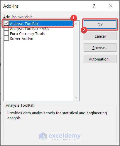
- Check the option Analysis ToolPak >> click OK.
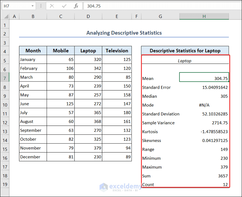
2.10.1. Analyze Descriptive Statistics
Now we will do some analysis with the sales quantity of laptops.
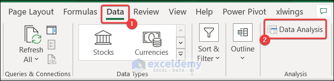
- Go to the Data tab >> Data Analysis.
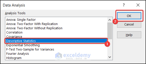
- Data Analysis dialog box will appear.
- Select Descriptive Statistics >> press OK.
- Descriptive Statistics dialog box will appear.
- Set the input range, output range, and other properties as shown below.
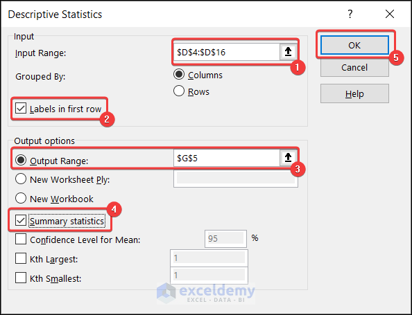
- You will see the descriptive statistics of laptop in your worksheet.
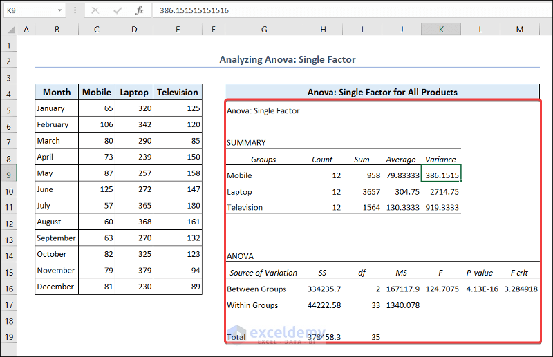
2.10.2. Analyze Anove: Single Factor
Now we will talk about the Anova analysis. Anova stands for Analysis of Variance. It is a statistical method to compare the means of two or more groups and determine if there is any significant difference between the groups.
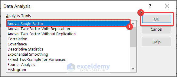
- Go to the Data tab >> Data Analysis.
- The Data Analysis dialog box will appear.
- Select Anova: Single Factor >> press OK.
- Anova: Single Factor window will appear.
- Set the input range, output range, and other properties as shown below.
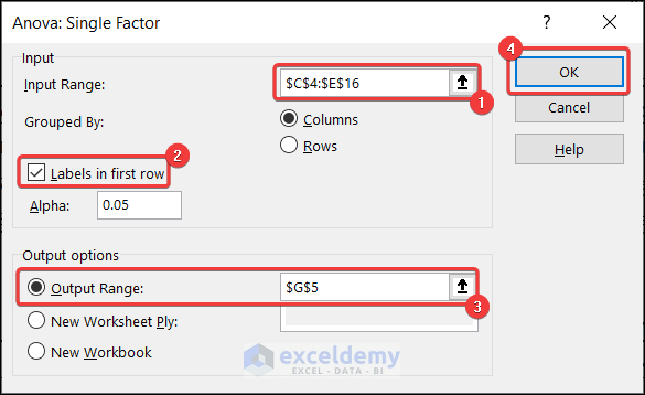
- You will find the analysis in your worksheet.
3. Data Visualization
After data analysis, we will try to visualize our dataset. Data visualization is the way to understand the pattern of the dataset. It also helps us to identify the outliers.
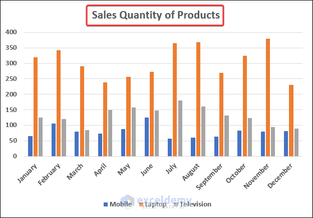
3.1. Excel Column Chart
- Select range B4:E16.
- Go to the Insert tab >> click on the columns icon drop-down >> select a suitable column chart.
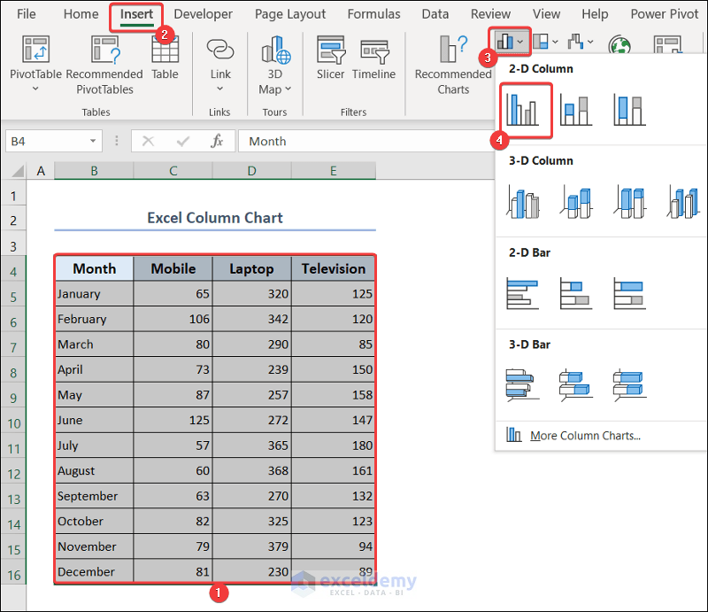
- You will have the column chart in your dataset. Give it a suitable title.
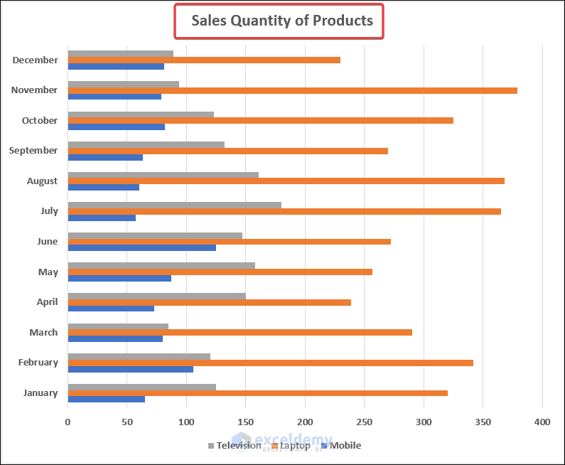
3.2. Excel Bar Chart
- Select range B4:E16.
- Go to the Insert tab >> click on the columns icon drop-down >> select a suitable bar chart.
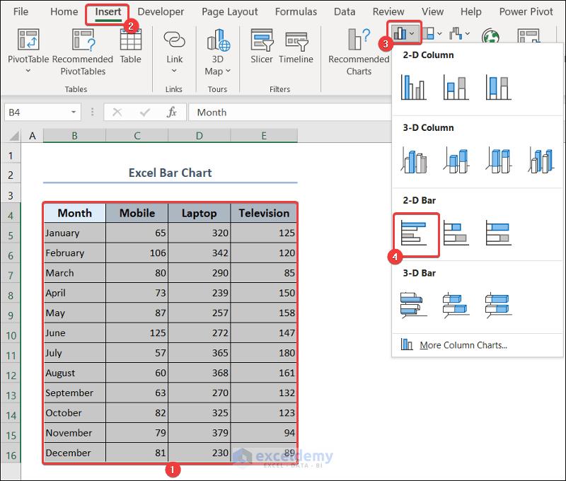
- You will have the bar chart in your dataset. Give it a suitable title.
3.3. Excel Line Chart
- Select range B4:E16.
- Go to the Insert tab >> click on the line chart icon drop-down.
- Select Line with Markers under the 2-D Line category.
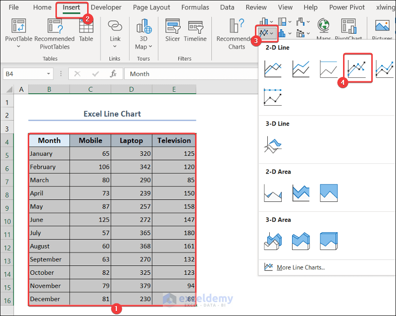
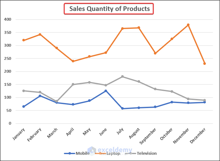
- You will have the line chart in your dataset. Give it a suitable title.
3.4. Excel Pie Chart
- Select range B4:C16.
- Go to the Insert tab >> click on the pie chart icon drop-down >> select an appropriate 2-D or 3-D pie chart.
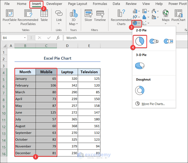
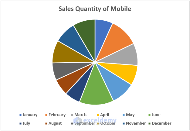
- You will see the pie chart showing the sales quantity of mobiles in your worksheet.
3.5. Excel Doughnut Chart
- Select range B4:B16 >> press the Ctrl button >> select range D4:D16.
- Go to the Insert tab >> click on the pie chart icon drop-down >> select the chart under the Doughnut category.
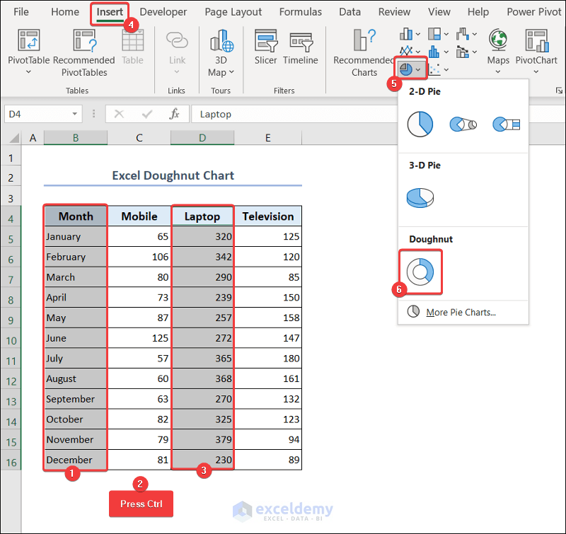
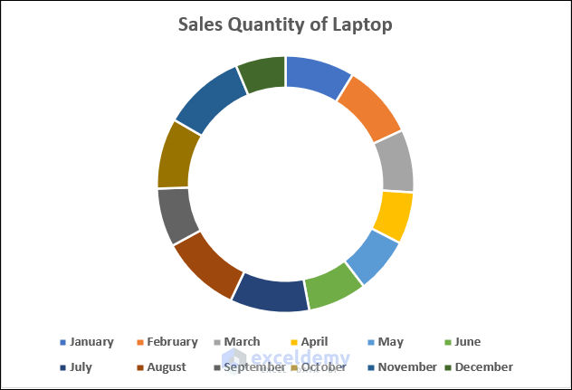
- You will see the doughnut chart showing the sales quantity of laptops in your worksheet.
Advanced Data Visualization
1. Excel Waterfall Chart
A waterfall chart is a unique chart that shows how positive and negative values contribute to the total. With waterfall charts, it is easy to understand the variation of values over a period of time. We will show you a waterfall chart for the sales quantity of televisions.
- Select range B4:B16 >> press the Ctrl button >> select range E4:E16.
- Go to the Insert tab >> click on the waterfall chart drop-down >> select the chart under the Waterfall category.
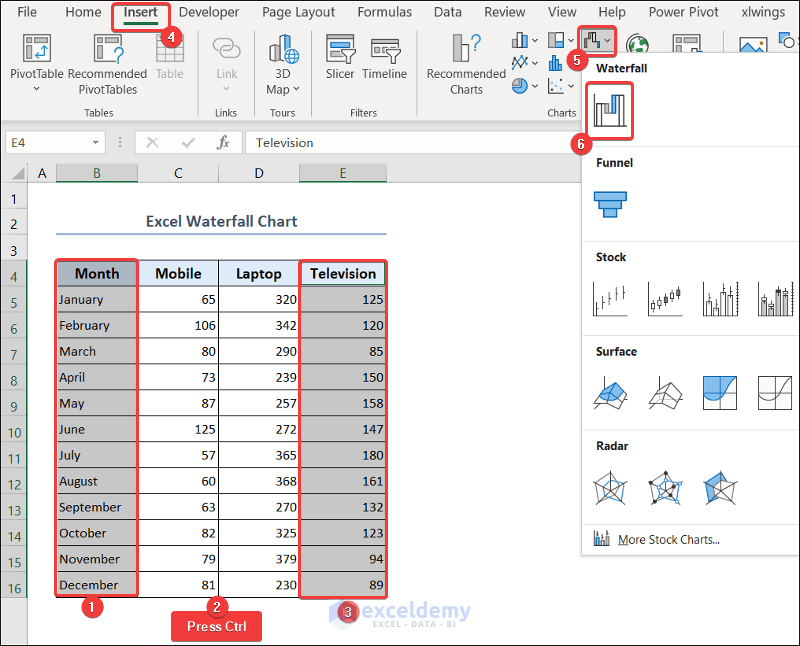
- You will see the waterfall chart showing the sales quantity of televisions.
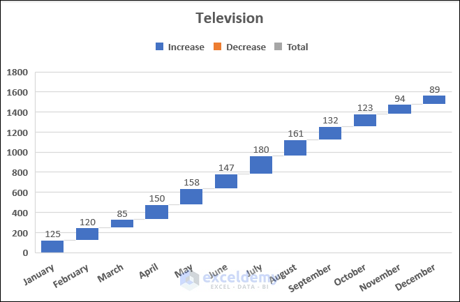
You will see only an increasing trend in this example because there are no negative values here. This chart is great for analyzing financial data over a period of time.
2. Animated Column Chart
Animated column chart displays data dynamically with animation effects. It does not create a static chart but rather the chart elements change or update over time, making it easier for you to understand the trend or pattern or the data points.
- Go to the Animated Chart worksheet.
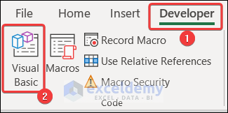
- Go to the Developer tab >> Visual Basic.
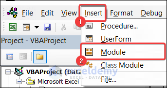
- Select Insert >> Module.
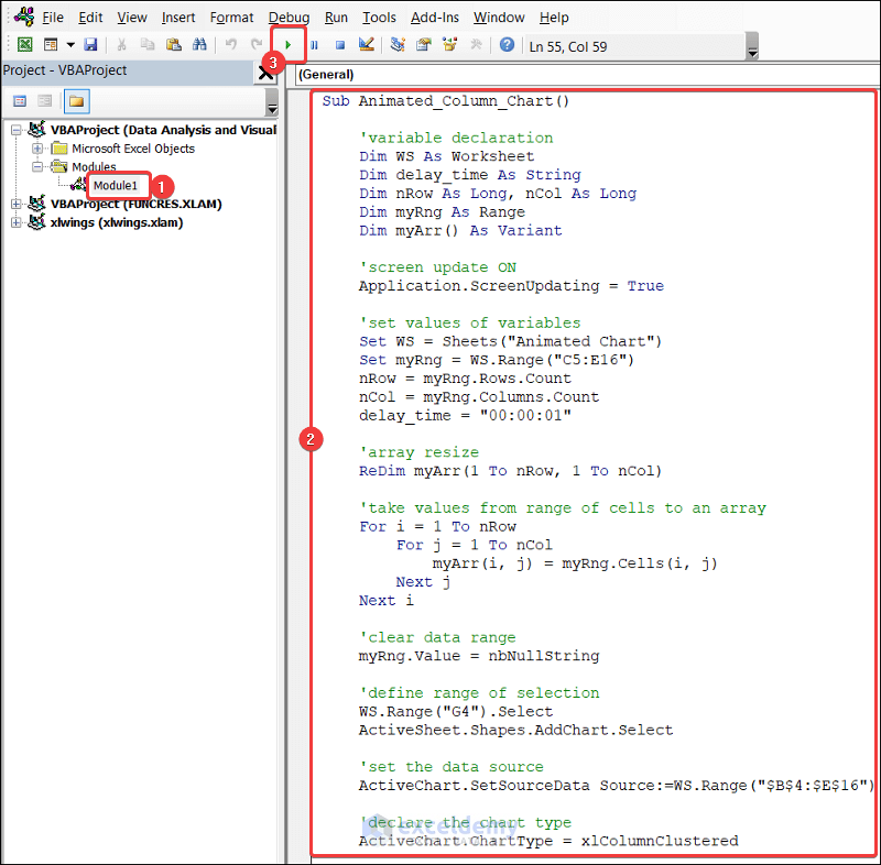
- Paste the following code in your VBA Macro Editor.
- Press the Run button or F5 key to run the code.
Sub Animated_Column_Chart()
    'variable declaration
    Dim WS As Worksheet
    Dim delay_time As String
    Dim nRow As Long, nCol As Long
    Dim myRng As Range
    Dim myArr() As Variant
    'screen update ON
    Application.ScreenUpdating = True
    'set values of variables
    Set WS = Sheets("Animated Chart")
    Set myRng = WS.Range("C5:E16")
    nRow = myRng.Rows.Count
    nCol = myRng.Columns.Count
    delay_time = "00:00:01"
    'array resize
    ReDim myArr(1 To nRow, 1 To nCol)
    'take values from range of cells to an array
    For i = 1 To nRow
        For j = 1 To nCol
            myArr(i, j) = myRng.Cells(i, j)
        Next j
    Next i
    'clear data range
    myRng.Value = nbNullString
    'define range of selection
    WS.Range("G4").Select
    ActiveSheet.Shapes.AddChart.Select
    'set the data source
    ActiveChart.SetSourceData Source:=WS.Range("$B$4:$E$16")
    'declare the chart type
    ActiveChart.ChartType = xlColumnClustered
    'declare activation command
    ActiveSheet.ChartObjects(1).Activate
    ActiveSheet.ChartObjects(1).Cut
    'select the chart destination
    WS.Select
    ActiveSheet.Paste
    'return to the worksheet
    WS.Select
    Range("B5").Activate
    'show values in range and create animated column chart race
    For i = 1 To nRow
        For j = 1 To nCol
            myRng.Cells(i, j) = myArr(i, j)
            DoEvents
        Next j
        DoEvents
        Application.Wait (Now + TimeValue(delay_time))
    Next i
End Sub- You will see the animated column chart in the Animated Chart worksheet.
VBA Breakdown
For i = 1 To nRow
        For j = 1 To nCol
            myArr(i, j) = myRng.Cells(i, j)
        Next j
Next i- These nested loops go through and copy values from myRng range to myArr array, one by one.
WS.Range("G4").Select
ActiveSheet.Shapes.AddChart.Select- These lines select cell G4 in the Animated Chart worksheet and add a new chart to the sheet.
ActiveChart.ChartType = xlColumnClustered- This line sets the chart type to a clustered column chart.
ActiveSheet.ChartObjects(1).Activate
    ActiveSheet.ChartObjects(1).Cut
    WS.Select
ActiveSheet.Paste- These lines activate the chart object, cut, and paste it into the Animated Chart worksheet.
For i = 1 To nRow
        For j = 1 To nCol
            myRng.Cells(i, j) = myArr(i, j)
            DoEvents
        Next j
        DoEvents
        Application.Wait (Now + TimeValue(delay_time))
Next i- These nested loops iterate through each cell in the myRng range and set its value from the myArr array. After setting each value, the DoEvents function allows the system to process events and update the screen to show the changes. Then, there is a time delay specified by the delay_time variable before moving to the next row. This is how animated chart effect is created.
Things to Remember
There are a few things to remember in data analysis and visualization with Excel.
- Instead of typing from a list, use Data Validation to ensure accurate data entry.
- Refresh your pivot table whenever you update your dataset.
- While using Data Analysis add-in, be careful with the selection of your input and output range.
Frequently Asked Questions
1. Why should I use Anova?
Anova is used to compare the trend difference between multiple datasets. It shows the variation of averages between multiple groups, how categorical variables affect outcome, and analyzes the validity of the given dataset. So, it is very useful for data analysis.
2. What is the difference between inferential and descriptive statistics?
Inferential statistics make predictions about a large group with a relatively smaller dataset. On the other hand, descriptive statistics describe various parameters of a dataset by summarizing it.
3. What is the advantage of using the Analyze Data feature?
Analyze Data feature comes with a lot of useful functions and tools, customizable capabilities, user friendly interface, and automated calculation techniques. It is much more flexible and far better than manual data analysis techniques.
Conclusion
In this article, we have explored data analysis and visualization with Excel in detail. By mastering these techniques, you can confidently analyze and visualize your data. If you have any questions regarding this essay, don’t hesitate to let us know in the comments. Also, if you want to see more Excel content like this, please visit our website, and unlock a great resource for Excel-related content.
Get FREE Advanced Excel Exercises with Solutions!
